Working with Data

Author

Alessandro Barberis

Published

May 16, 2026

1 Objective

In this lab we will work with a real clinical dataset from a prostate cancer cohort. By the end of the session you will be able to:

import a tabular dataset into R
explore its structure and contents
create basic visualisations with ggplot2
save your plots to disk

We introduce ggplot2 here as a practical tool. In later labs we will use it extensively, so it is worth getting comfortable with its core syntax now.

2 Setup

2.1 Project structure

This lab assumes you are working inside the course RStudio project. The project uses the here package to construct file paths relative to the project root, so the code works regardless of where you have saved the project on your computer.

If you do not have here or ggplot2 installed, run the chunk below once:

install.packages(c("here", "ggplot2"))

library(here)
library(ggplot2)

2.2 The `here` package

here::here() always returns the path to the project root, no matter which subfolder your .qmd file is in. For example:

# Shows the project root on your machine
here::here()

[1] "/home/runner/work/ai-clinical-research/ai-clinical-research"

All file paths in this document are built with here(), so you never need to adjust them manually.

3 Dataset: TCGA Prostate Cancer

3.1 About the data

We use clinical data from the Prostate Adenocarcinoma cohort of The Cancer Genome Atlas (TCGA), as curated in the TCGA PanCancer Atlas 2018. This cohort includes 499 patients with matched genomic and clinical data.

cBioPortal is an open-access platform that provides interactive exploration of large-scale cancer genomics datasets. It is widely used in translational oncology research and is a key resource you will encounter throughout this master.

3.2 Download the data

Go to the TCGA Prostate Cancer study page on cBioPortal.
Click Download.
Unzip the downloaded archive and move the folder prad_tcga_pan_can_atlas_2018/ into the data/ folder of the course project.

The file we need is data_clinical_patient.txt inside that folder.

Note

The dataset is already available in the data/ folder if you downloaded the full course materials from GitHub.

4 Import data

The clinical file uses tab-separated values with a 4-line header that describes the columns. We skip those lines and read the actual data starting at line 5.

clinical_data <- read.csv(
  file             = here("data", "prad_tcga_pan_can_atlas_2018", "data_clinical_patient.txt"),
  header           = TRUE,
  skip             = 4,
  sep              = "\t",
  stringsAsFactors = FALSE
)

5 Explore data

Before plotting or modelling, always explore your data. A few quick checks can save hours of debugging later.

# Preview the first 6 rows
head(clinical_data)

    PATIENT_ID SUBTYPE CANCER_TYPE_ACRONYM                     OTHER_PATIENT_ID
1 TCGA-2A-A8VL    PRAD                PRAD 49197847-CC83-4CE1-8397-D09CEA4C4928
2 TCGA-2A-A8VO    PRAD                PRAD 91C0D161-2B59-4B7A-8C19-6D26DEA31849
3 TCGA-2A-A8VT    PRAD                PRAD 931B549F-B9F2-4E8D-83ED-FF663671883C
4 TCGA-2A-A8VV    PRAD                PRAD 75A7AFB5-66D5-47E3-8A8A-3E3A1E749A96
5 TCGA-2A-A8VX    PRAD                PRAD 942F1788-D977-4AC0-A177-659F9D4CD077
6 TCGA-2A-A8W1    PRAD                PRAD F5319FD5-BEAE-4CA8-8F42-45FCA5E6A2D2
  AGE  SEX AJCC_PATHOLOGIC_TUMOR_STAGE AJCC_STAGING_EDITION DAYS_LAST_FOLLOWUP
1  51 Male                          NA                   NA                621
2  57 Male                          NA                   NA               1701
3  47 Male                          NA                   NA               1373
4  52 Male                          NA                   NA                671
5  70 Male                          NA                   NA               1378
6  54 Male                          NA                   NA                112
  DAYS_TO_BIRTH DAYS_TO_INITIAL_PATHOLOGIC_DIAGNOSIS ETHNICITY
1        -18658                                    0          
2        -20958                                    0          
3        -17365                                    0          
4        -19065                                    0          
5        -25904                                    0          
6        -19964                                    0          
  FORM_COMPLETION_DATE HISTORY_NEOADJUVANT_TRTYN ICD_10 ICD_O_3_HISTOLOGY
1              3/29/14                        No    C61            8140/3
2              3/30/14                        No    C61            8140/3
3              3/29/14                        No    C61            8140/3
4              3/29/14                        No    C61            8140/3
5              3/29/14                        No    C61            8140/3
6              3/29/14                        No    C61            8140/3
  ICD_O_3_SITE INFORMED_CONSENT_VERIFIED
1        C61.9                       Yes
2        C61.9                       Yes
3        C61.9                       Yes
4        C61.9                       Yes
5        C61.9                       Yes
6        C61.9                       Yes
  NEW_TUMOR_EVENT_AFTER_INITIAL_TREATMENT PATH_M_STAGE PATH_N_STAGE
1                                      No           NA           N0
2                                      No           NA             
3                                      No           NA           N1
4                                      No           NA           N0
5                                      No           NA           N0
6                                      No           NA           N0
  PATH_T_STAGE PERSON_NEOPLASM_CANCER_STATUS
1          T2B                    Tumor Free
2          T3A                    Tumor Free
3           T4                    Tumor Free
4          T2B                    Tumor Free
5          T3B                    Tumor Free
6          T3A                              
  PRIMARY_LYMPH_NODE_PRESENTATION_ASSESSMENT PRIOR_DX RACE RADIATION_THERAPY
1                                         NA       No                     No
2                                         NA       No                     No
3                                         NA       No                    Yes
4                                         NA       No                     No
5                                         NA       No                     No
6                                         NA       No                       
  WEIGHT IN_PANCANPATHWAYS_FREEZE OS_STATUS OS_MONTHS
1     NA                      Yes  0:LIVING 20.416215
2     NA                      Yes  0:LIVING 55.922675
3     NA                      Yes  0:LIVING 45.139231
4     NA                      Yes  0:LIVING 22.060032
5     NA                      Yes  0:LIVING 45.303613
6     NA                      Yes  0:LIVING  3.682151
                  DSS_STATUS DSS_MONTHS DFS_STATUS DFS_MONTHS PFS_STATUS
1 0:ALIVE OR DEAD TUMOR FREE  20.416215                    NA 0:CENSORED
2 0:ALIVE OR DEAD TUMOR FREE  55.922675                    NA 0:CENSORED
3 0:ALIVE OR DEAD TUMOR FREE  45.139231                    NA 0:CENSORED
4 0:ALIVE OR DEAD TUMOR FREE  22.060032                    NA 0:CENSORED
5 0:ALIVE OR DEAD TUMOR FREE  45.303613                    NA 0:CENSORED
6 0:ALIVE OR DEAD TUMOR FREE   3.682151                    NA 0:CENSORED
  PFS_MONTHS GENETIC_ANCESTRY_LABEL
1  20.416215                       
2  55.922675                    EUR
3  45.139231              SAS_ADMIX
4  22.060032                  ADMIX
5  45.303613                    EUR
6   3.682151                    EAS

# Column names, types, and a sample of values
str(clinical_data)

'data.frame':   494 obs. of  38 variables:
 $ PATIENT_ID                                : chr  "TCGA-2A-A8VL" "TCGA-2A-A8VO" "TCGA-2A-A8VT" "TCGA-2A-A8VV" ...
 $ SUBTYPE                                   : chr  "PRAD" "PRAD" "PRAD" "PRAD" ...
 $ CANCER_TYPE_ACRONYM                       : chr  "PRAD" "PRAD" "PRAD" "PRAD" ...
 $ OTHER_PATIENT_ID                          : chr  "49197847-CC83-4CE1-8397-D09CEA4C4928" "91C0D161-2B59-4B7A-8C19-6D26DEA31849" "931B549F-B9F2-4E8D-83ED-FF663671883C" "75A7AFB5-66D5-47E3-8A8A-3E3A1E749A96" ...
 $ AGE                                       : int  51 57 47 52 70 54 69 57 57 56 ...
 $ SEX                                       : chr  "Male" "Male" "Male" "Male" ...
 $ AJCC_PATHOLOGIC_TUMOR_STAGE               : logi  NA NA NA NA NA NA ...
 $ AJCC_STAGING_EDITION                      : logi  NA NA NA NA NA NA ...
 $ DAYS_LAST_FOLLOWUP                        : int  621 1701 1373 671 1378 112 863 1364 1272 615 ...
 $ DAYS_TO_BIRTH                             : int  -18658 -20958 -17365 -19065 -25904 -19964 -25557 -20866 -21183 -20582 ...
 $ DAYS_TO_INITIAL_PATHOLOGIC_DIAGNOSIS      : int  0 0 0 0 0 0 0 0 0 0 ...
 $ ETHNICITY                                 : chr  "" "" "" "" ...
 $ FORM_COMPLETION_DATE                      : chr  "3/29/14" "3/30/14" "3/29/14" "3/29/14" ...
 $ HISTORY_NEOADJUVANT_TRTYN                 : chr  "No" "No" "No" "No" ...
 $ ICD_10                                    : chr  "C61" "C61" "C61" "C61" ...
 $ ICD_O_3_HISTOLOGY                         : chr  "8140/3" "8140/3" "8140/3" "8140/3" ...
 $ ICD_O_3_SITE                              : chr  "C61.9" "C61.9" "C61.9" "C61.9" ...
 $ INFORMED_CONSENT_VERIFIED                 : chr  "Yes" "Yes" "Yes" "Yes" ...
 $ NEW_TUMOR_EVENT_AFTER_INITIAL_TREATMENT   : chr  "No" "No" "No" "No" ...
 $ PATH_M_STAGE                              : logi  NA NA NA NA NA NA ...
 $ PATH_N_STAGE                              : chr  "N0" "" "N1" "N0" ...
 $ PATH_T_STAGE                              : chr  "T2B" "T3A" "T4" "T2B" ...
 $ PERSON_NEOPLASM_CANCER_STATUS             : chr  "Tumor Free" "Tumor Free" "Tumor Free" "Tumor Free" ...
 $ PRIMARY_LYMPH_NODE_PRESENTATION_ASSESSMENT: logi  NA NA NA NA NA NA ...
 $ PRIOR_DX                                  : chr  "No" "No" "No" "No" ...
 $ RACE                                      : chr  "" "" "" "" ...
 $ RADIATION_THERAPY                         : chr  "No" "No" "Yes" "No" ...
 $ WEIGHT                                    : logi  NA NA NA NA NA NA ...
 $ IN_PANCANPATHWAYS_FREEZE                  : chr  "Yes" "Yes" "Yes" "Yes" ...
 $ OS_STATUS                                 : chr  "0:LIVING" "0:LIVING" "0:LIVING" "0:LIVING" ...
 $ OS_MONTHS                                 : num  20.4 55.9 45.1 22.1 45.3 ...
 $ DSS_STATUS                                : chr  "0:ALIVE OR DEAD TUMOR FREE" "0:ALIVE OR DEAD TUMOR FREE" "0:ALIVE OR DEAD TUMOR FREE" "0:ALIVE OR DEAD TUMOR FREE" ...
 $ DSS_MONTHS                                : num  20.4 55.9 45.1 22.1 45.3 ...
 $ DFS_STATUS                                : chr  "" "" "" "" ...
 $ DFS_MONTHS                                : num  NA NA NA NA NA ...
 $ PFS_STATUS                                : chr  "0:CENSORED" "0:CENSORED" "0:CENSORED" "0:CENSORED" ...
 $ PFS_MONTHS                                : num  20.4 55.9 45.1 22.1 45.3 ...
 $ GENETIC_ANCESTRY_LABEL                    : chr  " " "EUR" "SAS_ADMIX" "ADMIX" ...

# Statistical summary of each column
summary(clinical_data)

  PATIENT_ID          SUBTYPE          CANCER_TYPE_ACRONYM OTHER_PATIENT_ID  
 Length:494         Length:494         Length:494          Length:494        
 Class :character   Class :character   Class :character    Class :character  
 Mode  :character   Mode  :character   Mode  :character    Mode  :character  
                                                                             
                                                                             
                                                                             
                                                                             
      AGE            SEX            AJCC_PATHOLOGIC_TUMOR_STAGE
 Min.   :41.00   Length:494         Mode:logical               
 1st Qu.:56.00   Class :character   NA's:494                   
 Median :61.00   Mode  :character                              
 Mean   :61.02                                                 
 3rd Qu.:66.00                                                 
 Max.   :78.00                                                 
                                                               
 AJCC_STAGING_EDITION DAYS_LAST_FOLLOWUP DAYS_TO_BIRTH   
 Mode:logical         Min.   :   0.0     Min.   :-28721  
 NA's:494             1st Qu.: 517.5     1st Qu.:-24294  
                      Median : 924.0     Median :-22626  
                      Mean   :1080.1     Mean   :-22487  
                      3rd Qu.:1463.2     3rd Qu.:-20746  
                      Max.   :5024.0     Max.   :-15330  
                      NA's   :8          NA's   :11      
 DAYS_TO_INITIAL_PATHOLOGIC_DIAGNOSIS  ETHNICITY         FORM_COMPLETION_DATE
 Min.   :0                            Length:494         Length:494          
 1st Qu.:0                            Class :character   Class :character    
 Median :0                            Mode  :character   Mode  :character    
 Mean   :0                                                                   
 3rd Qu.:0                                                                   
 Max.   :0                                                                   
 NA's   :31                                                                  
 HISTORY_NEOADJUVANT_TRTYN    ICD_10          ICD_O_3_HISTOLOGY 
 Length:494                Length:494         Length:494        
 Class :character          Class :character   Class :character  
 Mode  :character          Mode  :character   Mode  :character  
                                                                
                                                                
                                                                
                                                                
 ICD_O_3_SITE       INFORMED_CONSENT_VERIFIED
 Length:494         Length:494               
 Class :character   Class :character         
 Mode  :character   Mode  :character         
                                             
                                             
                                             
                                             
 NEW_TUMOR_EVENT_AFTER_INITIAL_TREATMENT PATH_M_STAGE   PATH_N_STAGE      
 Length:494                              Mode:logical   Length:494        
 Class :character                        NA's:494       Class :character  
 Mode  :character                                       Mode  :character  
                                                                          
                                                                          
                                                                          
                                                                          
 PATH_T_STAGE       PERSON_NEOPLASM_CANCER_STATUS
 Length:494         Length:494                   
 Class :character   Class :character             
 Mode  :character   Mode  :character             
                                                 
                                                 
                                                 
                                                 
 PRIMARY_LYMPH_NODE_PRESENTATION_ASSESSMENT   PRIOR_DX        
 Mode:logical                               Length:494        
 NA's:494                                   Class :character  
                                            Mode  :character  
                                                              
                                                              
                                                              
                                                              
     RACE           RADIATION_THERAPY   WEIGHT        IN_PANCANPATHWAYS_FREEZE
 Length:494         Length:494         Mode:logical   Length:494              
 Class :character   Class :character   NA's:494       Class :character        
 Mode  :character   Mode  :character                  Mode  :character        
                                                                              
                                                                              
                                                                              
                                                                              
  OS_STATUS           OS_MONTHS         DSS_STATUS          DSS_MONTHS      
 Length:494         Min.   :  0.7562   Length:494         Min.   :  0.7562  
 Class :character   1st Qu.: 17.2272   Class :character   1st Qu.: 17.2272  
 Mode  :character   Median : 30.3777   Mode  :character   Median : 30.3777  
                    Mean   : 35.7313                      Mean   : 35.7313  
                    3rd Qu.: 48.1063                      3rd Qu.: 48.1063  
                    Max.   :165.1708                      Max.   :165.1708  
                                                                            
  DFS_STATUS          DFS_MONTHS       PFS_STATUS          PFS_MONTHS      
 Length:494         Min.   :  1.874   Length:494         Min.   :  0.7562  
 Class :character   1st Qu.: 19.413   Class :character   1st Qu.: 13.8327  
 Mode  :character   Median : 30.328   Mode  :character   Median : 25.6929  
                    Mean   : 35.657                      Mean   : 31.6613  
                    3rd Qu.: 45.665                      3rd Qu.: 44.7940  
                    Max.   :165.171                      Max.   :165.1708  
                    NA's   :160                                            
 GENETIC_ANCESTRY_LABEL
 Length:494            
 Class :character      
 Mode  :character

What to look for

When exploring a new dataset, pay attention to:

Missing values (NA): summary() reports their count per column.
Unexpected types: a numeric column stored as character is a common import issue.
Implausible values: e.g. a patient age of 0 or 999 usually signals a coding convention for missing data.

6 Visualise data with `ggplot2`

ggplot2 implements the Grammar of Graphics: every plot is built by combining a dataset, an aesthetic mapping (which variables map to x, y, colour, etc.), and one or more geometric layers (points, lines, bars, etc.).

The basic template is always:

ggplot(data, aes(x = ..., y = ...)) +
  geom_*() +
  labs(...)

6.1 Scatter plot: age vs. follow-up duration

ggplot(clinical_data, aes(x = AGE, y = DAYS_LAST_FOLLOWUP)) +
  geom_point(alpha = 0.5) +
  labs(
    title = "Age at diagnosis vs. days to last follow-up",
    x     = "Age at diagnosis (years)",
    y     = "Days to last follow-up"
  )

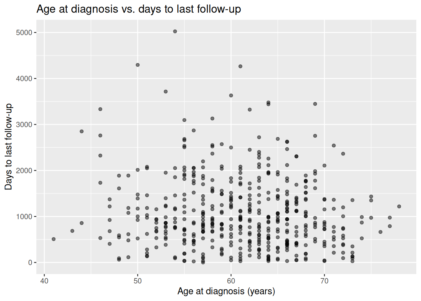
This plot shows the relationship between age at diagnosis and the length of follow-up. Each point is one patient. The alpha argument controls point transparency, which helps reveal overplotted regions.

7 Save a plot

Use ggsave() to export the last plot to a file. Specifying width, height, and dpi ensures consistent, publication-quality output.

ggsave(
  filename = here("output", "scatter_age_followup.png"),
  plot     = last_plot(),
  width    = 8,
  height   = 6,
  dpi      = 300
)

Note

The output/ folder must exist before running this chunk. Create it in the Files pane of RStudio, or run dir.create(here("output")) once.

8 Exercises

Work through the exercises below. Try to write the code yourself before looking at the solution.

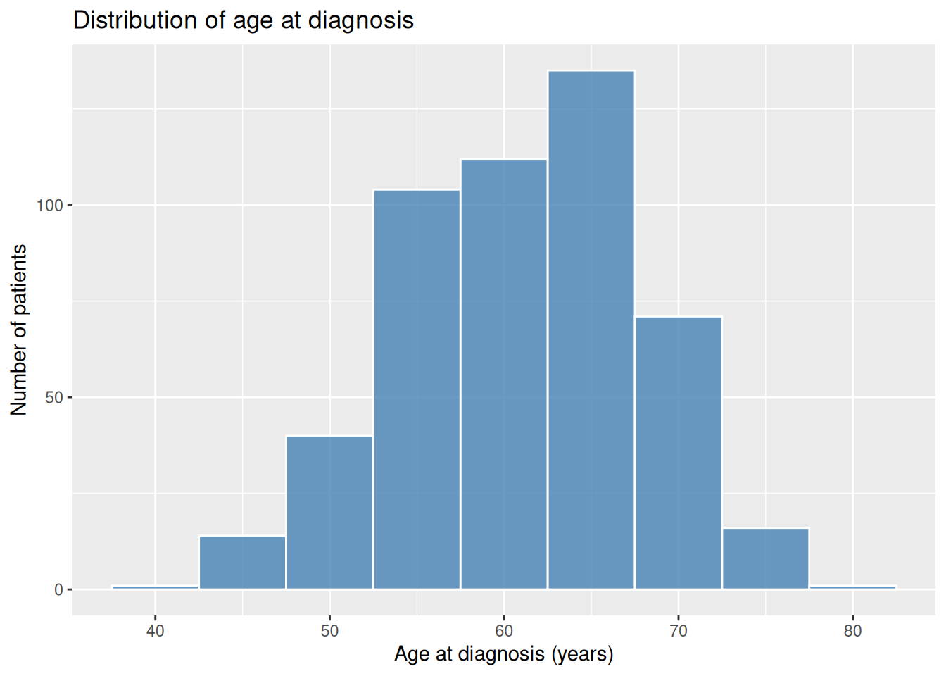
8.1 Exercise 1: Distribution of age at diagnosis

Create a histogram showing the distribution of patient age at diagnosis.

Hint: look at the ggplot2 documentation for geom_histogram(). Try adjusting the binwidth argument to see how it affects the plot.

# Your code here

Solution

ggplot(clinical_data, aes(x = AGE)) +
  geom_histogram(binwidth = 5, fill = "steelblue", color = "white", alpha = 0.8) +
  labs(
    title = "Distribution of age at diagnosis",
    x     = "Age at diagnosis (years)",
    y     = "Number of patients"
  )

8.2 Exercise 2: Overall survival by pathological stage

Create a violin plot showing the distribution of overall survival time (in months) for each pathological T-stage.

Hints:

Look at geom_violin() in the ggplot2 documentation.
Add a geom_jitter() layer on top to show individual data points.
The relevant columns are PATH_T_STAGE and OS_MONTHS.

# Your code here

Solution

ggplot(clinical_data, aes(x = PATH_T_STAGE, y = OS_MONTHS)) +
  geom_violin(fill = "lightblue", alpha = 0.6) +
  geom_jitter(width = 0.15, alpha = 0.4, size = 0.8) +
  labs(
    title = "Overall survival by pathological T-stage",
    x     = "Pathological T-stage",
    y     = "Overall survival (months)"
  )

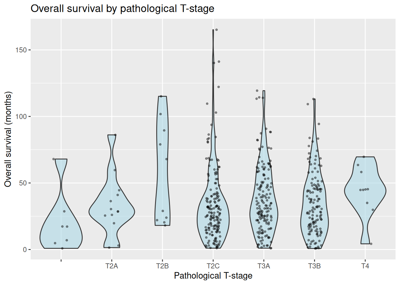
Notice how the violin plot reveals the shape of the distribution within each stage, while the jittered points show the actual density of observations.

8.3 Exercise 3 (optional): Kaplan–Meier survival curves

Going deeper: survival analysis

If you are familiar with survival analysis, try plotting Kaplan–Meier curves stratified by pathological stage using the survminer and survival packages.

# install.packages(c("survival", "survminer"))
library(survival)
library(survminer)

# Create a survival object
# OS_STATUS coding: check the data dictionary — typically 0 = alive, 1 = dead
surv_obj <- Surv(time = clinical_data$OS_MONTHS,
                 event = clinical_data$OS_STATUS == "DECEASED")

# Fit KM curves by pathological stage
km_fit <- survfit(surv_obj ~ PATH_T_STAGE, data = clinical_data)

# Plot
ggsurvplot(
  km_fit,
  data       = clinical_data,
  risk.table = TRUE,
  pval       = TRUE,
  title      = "Kaplan–Meier survival by pathological T-stage"
)

We will cover survival analysis in more detail in later sessions.

9 Session Info

sessionInfo()

R version 4.5.2 (2025-10-31)
Platform: x86_64-pc-linux-gnu
Running under: Ubuntu 24.04.4 LTS

Matrix products: default
BLAS:   /usr/lib/x86_64-linux-gnu/openblas-pthread/libblas.so.3 
LAPACK: /usr/lib/x86_64-linux-gnu/openblas-pthread/libopenblasp-r0.3.26.so;  LAPACK version 3.12.0

locale:
 [1] LC_CTYPE=C.UTF-8       LC_NUMERIC=C           LC_TIME=C.UTF-8       
 [4] LC_COLLATE=C.UTF-8     LC_MONETARY=C.UTF-8    LC_MESSAGES=C.UTF-8   
 [7] LC_PAPER=C.UTF-8       LC_NAME=C              LC_ADDRESS=C          
[10] LC_TELEPHONE=C         LC_MEASUREMENT=C.UTF-8 LC_IDENTIFICATION=C   

time zone: UTC
tzcode source: system (glibc)

attached base packages:
[1] stats     graphics  grDevices utils     datasets  methods   base     

other attached packages:
[1] ggplot2_4.0.3 here_1.0.2   

loaded via a namespace (and not attached):
 [1] vctrs_0.7.3        cli_3.6.6          knitr_1.51         rlang_1.2.0       
 [5] xfun_0.57          otel_0.2.0         generics_0.1.4     S7_0.2.2          
 [9] jsonlite_2.0.0     labeling_0.4.3     glue_1.8.1         rprojroot_2.1.1   
[13] htmltools_0.5.9    scales_1.4.0       rmarkdown_2.31     grid_4.5.2        
[17] tibble_3.3.1       evaluate_1.0.5     fastmap_1.2.0      yaml_2.3.12       
[21] lifecycle_1.0.5    compiler_4.5.2     dplyr_1.2.1        RColorBrewer_1.1-3
[25] pkgconfig_2.0.3    htmlwidgets_1.6.4  farver_2.1.2       digest_0.6.39     
[29] R6_2.6.1           tidyselect_1.2.1   pillar_1.11.1      magrittr_2.0.5    
[33] withr_3.0.2        tools_4.5.2        gtable_0.3.6

1 Objective

2 Setup

2.1 Project structure

2.2 The here package

3 Dataset: TCGA Prostate Cancer

3.1 About the data

3.2 Download the data

4 Import data

5 Explore data

6 Visualise data with ggplot2

6.1 Scatter plot: age vs. follow-up duration

7 Save a plot

8 Exercises

8.1 Exercise 1: Distribution of age at diagnosis

8.2 Exercise 2: Overall survival by pathological stage

8.3 Exercise 3 (optional): Kaplan–Meier survival curves

9 Session Info

2.2 The `here` package

6 Visualise data with `ggplot2`