Classification • renoir

Introduction

This article is used to benchmark the evaluations obtained by renoir for classification problems against external results.

Data

Different public datasets already used in classification problems are considered:

The breast cancer data from the University of Wisconsin Hospitals
The heart-disease data from the Cleveland Clinic Foundation

Data was retrieved from the UC Irvine Machine Learning Repository website.

Setup

Firstly, we load renoir and other needed packages:

library(renoir)
#> Warning: package 'Matrix' was built under R version 4.2.3
library(plotly)
library(htmltools)

Learning Methods

Now we retrieve the ids of all the supported learners. A list of supported methods is available through the ?list_supported_learning_methods function call.

#list methods
learning.methods = list_supported_learning_methods(x = "classification")

#print in table
knitr::kable(x = learning.methods)

id	method	default_hyperparameters
lasso	generalized linear model via L1 penalized maximum likelihood (lasso penalty)	lambda
ridge	generalized linear model via L2 penalized maximum likelihood (ridge penalty)	lambda
elasticnet	generalized linear model via L1/L2 penalized maximum likelihood (elasticnet penalty)	lambda, ….
relaxed_lasso	generalized linear model via L1 penalized maximum likelihood (relaxed lasso penalty)	lambda, ….
relaxed_ridge	generalized linear model via L2 penalized maximum likelihood (relaxed ridge penalty)	lambda, ….
relaxed_elasticnet	generalized linear model via L1/L2 penalized maximum likelihood (relaxed elasticnet penalty)	lambda, ….
randomForest	random forest	ntree
gbm	generalized boosted model	eta, ntree
linear_SVM	linear support vector machine	cost
polynomial_SVM	polynomial support vector machine	cost, ga….
radial_SVM	radial support vector machine	cost, gamma
sigmoid_SVM	sigmoid support vector machine	cost, gamma
linear_NuSVM	linear nu-type support vector machine	nu
polynomial_NuSVM	polynomial nu-type support vector machine	nu, gamm….
radial_NuSVM	radial nu-type support vector machine	nu, gamma
sigmoid_NuSVM	sigmoid nu-type support vector machine	nu, gamma
gknn	generalized k-nearest neighbours model	k
nsc	nearest shrunken centroid model	threshold

We can extract the ids by selecting the id column.

#learning method ids
learning.methods.ids = learning.methods$id

From the table, we can also see the default hyperparameters of the methods. We create here our default values, and define a function to dispatch them depending on the id in input:

#get hyperparameters
get_hp = function(id, y){

  #Generalised Linear Models with Penalisation
  lambda = 10^seq(3, -2, length=100)
  # alpha = seq(0.1, 0.9, length = 9)
  alpha = seq(0.1, 0.9, length = 5)
  gamma = c(0, 0.25, 0.5, 0.75, 1)
  
  #Random Forest
  ntree = c(10, 50, 100, 250, 500)
  
  #Generalised Boosted Regression Modelling
  eta = c(0.3, 0.1, 0.01, 0.001)
  
  #Support Vector Machines
  cost      = 2^seq(from = -5, to = 15, length.out = 5)
  svm.gamma = 2^seq(from = -15, to = 3, length.out = 4)
  degree    = seq(from = 1, to = 3, length.out = 3)
  #Note that for classification nu must be
  #nu * length(y)/2 <= min(table(y)). So instead of
  #fixing it as
  # nu        = seq(from = 0.1, to = 0.6, length.out = 5)
  #we do
  nu.to = floor((min(table(y)) * 2/length(y)) * 10) / 10
  nu = seq(from = 0.1, to = nu.to, length.out = 5)
  
  #kNN
  k = seq(from = 1, to = 9, length.out = 5)

  #Nearest Shrunken Centroid
  threshold = seq(0, 2, length.out = 30)

  #hyperparameters
  out = switch(
    id,
    'lasso'              = list(lambda = lambda),
    'ridge'              = list(lambda = lambda),
    'elasticnet'         = list(lambda = lambda, alpha = alpha),
    'relaxed_lasso'      = list(lambda = lambda, gamma = gamma),
    'relaxed_ridge'      = list(lambda = lambda, gamma = gamma),
    'relaxed_elasticnet' = list(lambda = lambda, gamma = gamma, alpha = alpha),
    'randomForest'       = list(ntree = ntree),
    'gbm'                = list(eta = eta, ntree = ntree),
    'linear_SVM'         = list(cost = cost),
    'polynomial_SVM'     = list(cost = cost, gamma = svm.gamma, degree = degree),
    'radial_SVM'         = list(cost = cost, gamma = svm.gamma),
    'sigmoid_SVM'        = list(cost = cost, gamma = svm.gamma),
    'linear_NuSVM'       = list(nu = nu),
    'polynomial_NuSVM'   = list(nu = nu, gamma = svm.gamma, degree = degree),
    'radial_NuSVM'       = list(nu = nu, gamma = svm.gamma),
    'sigmoid_NuSVM'      = list(nu = nu, gamma = svm.gamma),
    'gknn'               = list(k = k),
    'nsc'                = list(threshold = threshold)
  )

  return(out)
}

Performance metrics

A list of supported scoring metrics is available through the ?list_supported_performance_metrics function call.

#list metrics
performance.metrics = list_supported_performance_metrics(resp.type = "binomial")

#print in table
knitr::kable(x = performance.metrics)

id	name	problem
class	Misclassification Error	classification
acc	Accuracy	classification
auc	AUC	classification
f1s	F1 Score	classification
fbeta	F-beta Score	classification
precision	Precision	classification
sensitivity	Sensitivity	classification
jaccard	Jaccard Index	classification

For this benchmark we want to select accuracy and precision, as these are the reported measure on the website.

#metric for tuning
performance.metric.id.tuning = "acc"

#metrics for evaluation
performance.metric.ids.evaluation = c("acc", "precision")

Sampling Methods

A list of supported sampling methods is available through the ?list_supported_sampling_methods function call.

#list methods
sampling.methods = list_supported_sampling_methods()

#print in table
knitr::kable(x = sampling.methods)

id	name	supported
random	random sampling without replacement	stratification, balance
bootstrap	random sampling with replacement	stratification, balance
cv	cross-validation	stratification

We decided to select the common scenario of a stratified 10-fold cross-validation for the tuning of hyperparameters, and repeated random sampling for the evaluation of the methodology.

#sampling for tuning
sampling.method.id.tuning = "cv"

#sampling for evaluation
sampling.method.id.evaluation = "random"

Benchmark

We can now run our analyses.

Breast Cancer Data

The Breast Cancer database from the University of Wisconsin Hospitals was retrieved from the UC Irvine Machine Learning Repository website.

Load data

We load the data.

#load data
load(file = file.path("..", "..", "data-raw", "benchmark", "classification", "bcwo", "data", "bcwo_data.rda"))

We need to set the response type.

#set response type
resp.type = "binomial"

Setup

Tuner

Now we can create a tuner performing a grid.search via 10-fold cross-validation.

#tuner
tuner = Tuner(
  id = "grid.search",
  sampler = Sampler(
    method = sampling.method.id.tuning,
    k = 10L,
    n = integer(),
    strata = y
  ),
  looper   = Looper(cores = 1L),
  logger   = Logger(verbose = T, level = "INFO")
)

Learner

We can now create the related ?Learner objects.

#container
learners = list()

#loop
for(learning.method.id in learning.methods.ids){
  #manual setup
  learners[[learning.method.id]] = Learner(
    tuner      = tuner,
    trainer    = Trainer(id = learning.method.id),
    forecaster = Forecaster(id = learning.method.id),
    scorer     = ScorerList(Scorer(id = performance.metric.id.tuning)),
    selector   = Selector(id = learning.method.id),
    recorder   = Recorder(id = learning.method.id),
    marker     = Marker(id = learning.method.id),
    logger     = Logger(level = "ALL")
  )
}

Evaluator

Finally, we need to set up the ?Evaluator.

#Evaluator
evaluator = Evaluator(
  #Sampling strategy: stratified random sampling without replacement
  sampler = Sampler(               
    method = "random",             
    k = 10L,                       
    strata = y,                    
    N = as.integer(length(y))      
  ),

  #Performance metric
  scorer  = ScorerList(
    Scorer(id = performance.metric.ids.evaluation[1]),
    Scorer(id = performance.metric.ids.evaluation[2])
  )
)

Analysis

Let’s create a directory to store the results.


#define path
outdir = file.path("..", "..", "data-raw", "benchmark", "classification", "bcwo", "analysis")

#create if not existing
if(!dir.exists(outdir)){dir.create(path = outdir, showWarnings = F, recursive = T)}

Before running the analysis, we want to set a seed for the random number generation (RNG). In fact, different R sessions have different seeds created from current time and process ID by default, and consequently different simulation results. By fixing a seed we ensure we will be able to reproduce the results. We can specify a seed by calling ?set.seed.

In the code below, we set a seed before running the analysis for each considered learning method.

#container list
resl = list()

#loop
for(learning.method.id in learning.methods.ids){
  
  #Each analysis can take hours, so we save data 
  #for future faster load
  
  #path to file
  fp.obj = file.path(outdir, paste0(learning.method.id,".rds"))
  fp.sum = file.path(outdir, paste0("st_",learning.method.id,".rds"))
  
  #check if exists
  if(file.exists(fp.sum)){
    #load
    cat(paste0("Reading ", learning.method.id, "..."), sep = "")
    resl[[learning.method.id]] = readRDS(file = fp.sum)
    cat("DONE", sep = "\n")
  } else {
  
    cat(paste("Learning method:", learning.method.id), sep = "\n")
    
    #Set a seed for RNG
    set.seed(
      #A seed
      seed = 5381L,                   #a randomly chosen integer value
      #The kind of RNG to use
      kind = "Mersenne-Twister",      #we make explicit the current R default value
      #The kind of Normal generation
      normal.kind = "Inversion"       #we make explicit the current R default value
    )
    
    resl[[learning.method.id]] = renoir(
      # filter,
  
      #Training set size
      npoints = 5,
      # ngrid,
      nmin = round(nrow(x)/2),
  
      #Loop
      looper = Looper(),
  
      #Store
      filename = "renoir",
      outdir   = NULL,
      restore  = TRUE,
  
      #Learn
      learner   = learners[[learning.method.id]],
  
      #Evaluate
      evaluator = evaluator,
  
      #Log
      logger    = Logger(level = "ALL", verbose = T),
  
      #Data for training
      hyperparameters = get_hp(id = learning.method.id, y = y),
      x         = x,
      y         = y,
      weights   = NULL,
      offset    = NULL,
      resp.type = resp.type,
  
      #Free space
      rm.call = FALSE,
      rm.fit  = FALSE,
  
      #Group results
      grouping = TRUE,
  
      #No screening
      screening = NULL,
      
      #Remove call from trainer to reduce space
      keep.call = F
    )
    
    #save obj
    saveRDS(object = resl[[learning.method.id]], file = fp.obj)
    
    #create summary table
    resl[[learning.method.id]] = renoir:::summary_table.RenoirList(resl[[learning.method.id]], key = c("id", "config"))
    
    #save summary table
    saveRDS(object = resl[[learning.method.id]], file = fp.sum)
    
    cat("\n\n", sep = "\n")
  }
}

#create summary table
resl = do.call(what = rbind, args = c(resl, make.row.names = F, stringsAsFactors = F))

Performance

Let’s now plot the performance metrics for the opt and 1se configurations, considering the train, test, and full set of data.

Precision

We consider the precision.

Reference

This is the precision reported in the UC Irvine Machine Learning Repository website that we use as reference.

Train

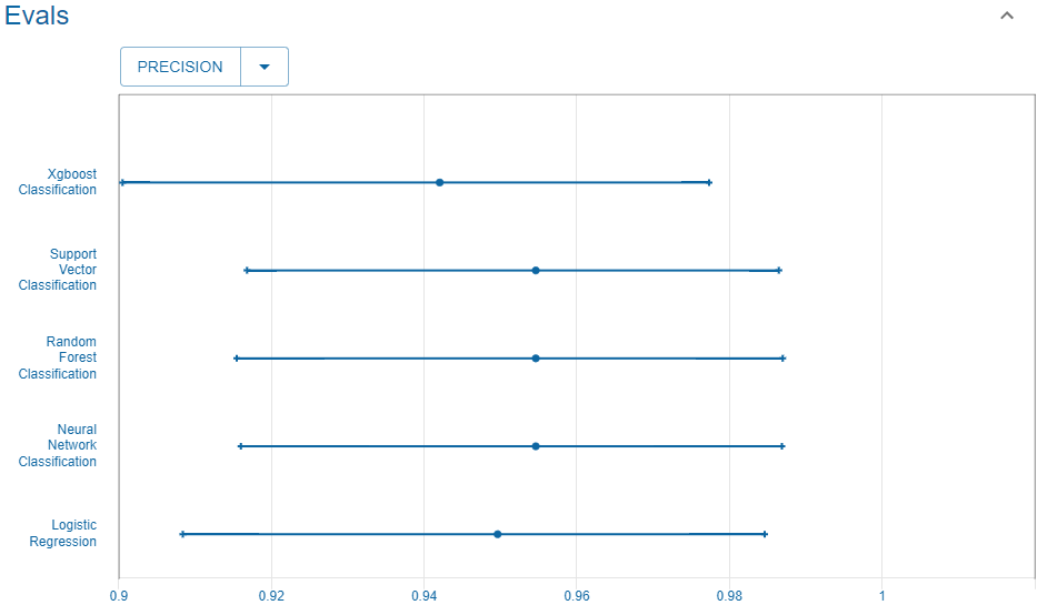
This is the precision score for the opt configuration when considering the train set.

#plot
renoir:::plot.RenoirSummaryTable(
  x = resl[resl$config == "opt",,drop=F],
  measure     = "precision", 
  set         = "train", 
  interactive = T, 
  add.boxplot = F,
  add.scores  = F,
  add.best    = F,
  key         = c("id", "config")
  )

#> Warning in RColorBrewer::brewer.pal(N, "Set2"): n too large, allowed maximum for palette Set2 is 8
#> Returning the palette you asked for with that many colors

#> Warning in RColorBrewer::brewer.pal(N, "Set2"): n too large, allowed maximum for palette Set2 is 8
#> Returning the palette you asked for with that many colors

This is the precision score for the 1se configuration when considering the train set.

#plot
renoir:::plot.RenoirSummaryTable(
  x = resl[resl$config == "1se",,drop=F], #select 1se config 
  measure     = "precision", 
  set         = "train", 
  interactive = T, 
  add.boxplot = F,
  add.scores  = F,
  add.best    = F,
  key         = c("id", "config")
  )

#> Warning in RColorBrewer::brewer.pal(N, "Set2"): n too large, allowed maximum for palette Set2 is 8
#> Returning the palette you asked for with that many colors

#> Warning in RColorBrewer::brewer.pal(N, "Set2"): n too large, allowed maximum for palette Set2 is 8
#> Returning the palette you asked for with that many colors

Test

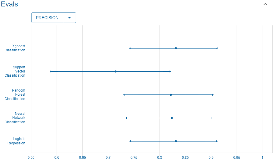
This is the precision score for the opt configuration when considering the test set.

#plot
renoir:::plot.RenoirSummaryTable(
  x = resl[resl$config == "opt",,drop=F], #select opt config
  measure     = "precision", 
  set         = "test", 
  interactive = T, 
  add.boxplot = F,
  add.scores  = F,
  add.best    = F,
  key         = c("id", "config")
  )

#> Warning in RColorBrewer::brewer.pal(N, "Set2"): n too large, allowed maximum for palette Set2 is 8
#> Returning the palette you asked for with that many colors

#> Warning in RColorBrewer::brewer.pal(N, "Set2"): n too large, allowed maximum for palette Set2 is 8
#> Returning the palette you asked for with that many colors

This is the precision score for the 1se configuration when considering the test set.

#plot
renoir:::plot.RenoirSummaryTable(
  x = resl[resl$config == "1se",,drop=F], #select 1se config 
  measure     = "precision", 
  set         = "test", 
  interactive = T, 
  add.boxplot = F,
  add.scores  = F,
  add.best    = F,
  key         = c("id", "config")
  )

#> Warning in RColorBrewer::brewer.pal(N, "Set2"): n too large, allowed maximum for palette Set2 is 8
#> Returning the palette you asked for with that many colors

#> Warning in RColorBrewer::brewer.pal(N, "Set2"): n too large, allowed maximum for palette Set2 is 8
#> Returning the palette you asked for with that many colors

Full

This is the precision score for the opt configuration when considering the full set.

#plot
renoir:::plot.RenoirSummaryTable(
  x = resl[resl$config == "opt",,drop=F], #select opt config
  measure     = "precision", 
  set         = "full", 
  interactive = T, 
  add.boxplot = F,
  add.scores  = F,
  add.best    = F,
  key         = c("id", "config")
  )

#> Warning in RColorBrewer::brewer.pal(N, "Set2"): n too large, allowed maximum for palette Set2 is 8
#> Returning the palette you asked for with that many colors

#> Warning in RColorBrewer::brewer.pal(N, "Set2"): n too large, allowed maximum for palette Set2 is 8
#> Returning the palette you asked for with that many colors

This is the precision score for the 1se configuration when considering the full set.

#plot
renoir:::plot.RenoirSummaryTable(
  x = resl[resl$config == "1se",,drop=F], #select 1se config 
  measure     = "precision", 
  set         = "full", 
  interactive = T, 
  add.boxplot = F,
  add.scores  = F,
  add.best    = F,
  key         = c("id", "config")
  )

#> Warning in RColorBrewer::brewer.pal(N, "Set2"): n too large, allowed maximum for palette Set2 is 8
#> Returning the palette you asked for with that many colors

#> Warning in RColorBrewer::brewer.pal(N, "Set2"): n too large, allowed maximum for palette Set2 is 8
#> Returning the palette you asked for with that many colors

Accuracy

We consider here the accuracy score.

Reference

This is the accuracy reported in the UC Irvine Machine Learning Repository website that we use as reference.

Train

This is the accuracy score for the opt configuration when considering the train set.

#plot
renoir:::plot.RenoirSummaryTable(
  x = resl[resl$config == "opt",,drop=F], #select opt config
  measure     = "acc", 
  set         = "train", 
  interactive = T, 
  add.boxplot = F,
  add.scores  = F,
  add.best    = F,
  key         = c("id", "config")
  )

#> Warning in RColorBrewer::brewer.pal(N, "Set2"): n too large, allowed maximum for palette Set2 is 8
#> Returning the palette you asked for with that many colors

#> Warning in RColorBrewer::brewer.pal(N, "Set2"): n too large, allowed maximum for palette Set2 is 8
#> Returning the palette you asked for with that many colors

This is the accuracy score for the 1se configuration when considering the train set.

#plot
renoir:::plot.RenoirSummaryTable(
  x = resl[resl$config == "1se",,drop=F], #select 1se config 
  measure     = "acc", 
  set         = "train", 
  interactive = T, 
  add.boxplot = F,
  add.scores  = F,
  add.best    = F,
  key         = c("id", "config")
  )

#> Warning in RColorBrewer::brewer.pal(N, "Set2"): n too large, allowed maximum for palette Set2 is 8
#> Returning the palette you asked for with that many colors

#> Warning in RColorBrewer::brewer.pal(N, "Set2"): n too large, allowed maximum for palette Set2 is 8
#> Returning the palette you asked for with that many colors

Test

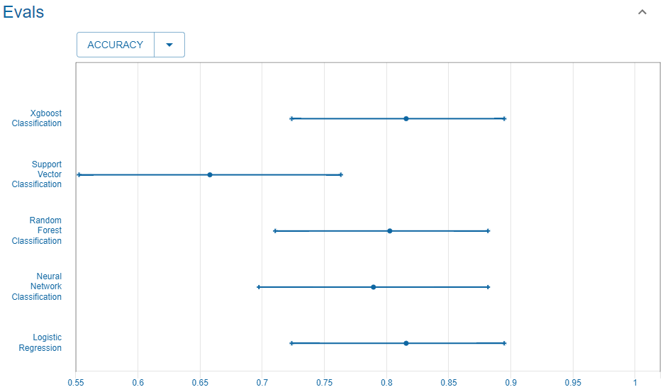
This is the accuracy score for the opt configuration when considering the test set.

#plot
renoir:::plot.RenoirSummaryTable(
  x = resl[resl$config == "opt",,drop=F], #select opt config
  measure     = "acc", 
  set         = "test", 
  interactive = T, 
  add.boxplot = F,
  add.scores  = F,
  add.best    = F,
  key         = c("id", "config")
  )

#> Warning in RColorBrewer::brewer.pal(N, "Set2"): n too large, allowed maximum for palette Set2 is 8
#> Returning the palette you asked for with that many colors

#> Warning in RColorBrewer::brewer.pal(N, "Set2"): n too large, allowed maximum for palette Set2 is 8
#> Returning the palette you asked for with that many colors

This is the accuracy score for the 1se configuration when considering the test set.

#plot
renoir:::plot.RenoirSummaryTable(
  x = resl[resl$config == "1se",,drop=F], #select 1se config 
  measure     = "acc", 
  set         = "test", 
  interactive = T, 
  add.boxplot = F,
  add.scores  = F,
  add.best    = F,
  key         = c("id", "config")
  )

#> Warning in RColorBrewer::brewer.pal(N, "Set2"): n too large, allowed maximum for palette Set2 is 8
#> Returning the palette you asked for with that many colors

#> Warning in RColorBrewer::brewer.pal(N, "Set2"): n too large, allowed maximum for palette Set2 is 8
#> Returning the palette you asked for with that many colors

Full

This is the accuracy score for the opt configuration when considering the full set.

#plot
renoir:::plot.RenoirSummaryTable(
  x = resl[resl$config == "opt",,drop=F], #select opt config
  measure     = "acc", 
  set         = "full", 
  interactive = T, 
  add.boxplot = F,
  add.scores  = F,
  add.best    = F,
  key         = c("id", "config")
  )

#> Warning in RColorBrewer::brewer.pal(N, "Set2"): n too large, allowed maximum for palette Set2 is 8
#> Returning the palette you asked for with that many colors

#> Warning in RColorBrewer::brewer.pal(N, "Set2"): n too large, allowed maximum for palette Set2 is 8
#> Returning the palette you asked for with that many colors

This is the accuracy score for the 1se configuration when considering the full set.

#plot
renoir:::plot.RenoirSummaryTable(
  x = resl[resl$config == "1se",,drop=F], #select 1se config 
  measure     = "acc", 
  set         = "full", 
  interactive = T, 
  add.boxplot = F,
  add.scores  = F,
  add.best    = F,
  key         = c("id", "config")
  )

#> Warning in RColorBrewer::brewer.pal(N, "Set2"): n too large, allowed maximum for palette Set2 is 8
#> Returning the palette you asked for with that many colors

#> Warning in RColorBrewer::brewer.pal(N, "Set2"): n too large, allowed maximum for palette Set2 is 8
#> Returning the palette you asked for with that many colors

Heart-Disease Data

The heart-disease database from the Cleveland Clinic Foundation was retrieved from the UC Irvine Machine Learning Repository website.

Load data

We load the data.

#load data
load(file = file.path("..", "..", "data-raw", "benchmark", "classification", "heart_disease", "data", "hdpc_data.rda"))

#set response type
resp.type = "binomial"

Setup

Tuner

Now we can create a tuner performing a grid.search via 10-fold cross-validation.

#tuner
tuner = Tuner(
  id = "grid.search",
  sampler = Sampler(
    method = sampling.method.id.tuning,
    k = 10L,
    n = integer(),
    strata = y
  ),
  looper   = Looper(cores = 1L),
  logger   = Logger(verbose = T, level = "INFO")
)

Learner

We can now create the related ?Learner objects.

#container
learners = list()

#loop
for(learning.method.id in learning.methods.ids){
  #manual setup
  learners[[learning.method.id]] = Learner(
    tuner      = tuner,
    trainer    = Trainer(id = learning.method.id),
    forecaster = Forecaster(id = learning.method.id),
    scorer     = ScorerList(Scorer(id = performance.metric.id.tuning)),
    selector   = Selector(id = learning.method.id),
    recorder   = Recorder(id = learning.method.id, logger = Logger(level = "ALL", verbose = T)),
    marker     = Marker(id = learning.method.id, logger = Logger(level = "ALL", verbose = T)),
    logger     = Logger(level = "ALL")
  )
}

Evaluator

Finally, we need to set up the ?Evaluator.

#Evaluator
evaluator = Evaluator(
  #Sampling strategy: stratified random sampling without replacement
  sampler = Sampler(               
    method = "random",             
    k = 10L,                       
    strata = y,                    
    N = as.integer(length(y))      
  ),

  #Performance metric
  scorer  = ScorerList(
    Scorer(id = performance.metric.ids.evaluation[1]),
    Scorer(id = performance.metric.ids.evaluation[2])
  )
)

Analysis

Let’s create a directory to store the results.

#define path
outdir = file.path("..", "..", "data-raw", "benchmark", "classification", "heart_disease", "analysis")

#create if not existing
if(!dir.exists(outdir)){dir.create(path = outdir, showWarnings = F, recursive = T)}

In the code below, we set a seed before running the analysis for each considered learning method.

#container list
resl = list()

#loop
for(learning.method.id in learning.methods.ids){
  
  #Each analysis can take hours, so we save data 
  #for future faster load
  
  #path to file
  fp.obj = file.path(outdir, paste0(learning.method.id,".rds"))#fit object
  fp.sum = file.path(outdir, paste0("st_",learning.method.id,".rds"))#summary table
  
  #check if exists
  if(file.exists(fp.sum)){
    #load
    cat(paste0("Reading ", learning.method.id, "..."), sep = "")
    resl[[learning.method.id]] = readRDS(file = fp.sum)
    cat("DONE", sep = "\n")
  } else {
  
    cat(paste("Learning method:", learning.method.id), sep = "\n")
    
    #Set a seed for RNG
    set.seed(
      #A seed
      seed = 5381L,                   #a randomly chosen integer value
      #The kind of RNG to use
      kind = "Mersenne-Twister",      #we make explicit the current R default value
      #The kind of Normal generation
      normal.kind = "Inversion"       #we make explicit the current R default value
    )
    
    resl[[learning.method.id]] = renoir(
      # filter,
  
      #Training set size
      npoints = 5,
      # ngrid,
      nmin = round(nrow(x)/2),
  
      #Loop
      looper = Looper(),
  
      #Store
      filename = "renoir",
      outdir   = NULL,
      restore  = TRUE,
  
      #Learn
      learner   = learners[[learning.method.id]],
  
      #Evaluate
      evaluator = evaluator,
  
      #Log
      logger    = Logger(level = "ALL", verbose = T),
  
      #Data for training
      hyperparameters = get_hp(id = learning.method.id, y = y),
      x         = x,
      y         = y,
      weights   = NULL,
      offset    = NULL,
      resp.type = resp.type,
  
      #space
      rm.call = FALSE,
      rm.fit  = FALSE,
  
      #Group results
      grouping = TRUE,
  
      #No screening
      screening = NULL,
      
      #Remove call from trainer to reduce space
      keep.call = F
    )
    
    #save
    saveRDS(object = resl[[learning.method.id]], file = fp.obj)
    
    #create summary table
    resl[[learning.method.id]] = renoir:::summary_table.RenoirList(resl[[learning.method.id]], key = c("id", "config"))
    
    #save summary table
    saveRDS(object = resl[[learning.method.id]], file = fp.sum)
    
    cat("\n\n", sep= "\n")
  }
}

#create summary table
resl = do.call(what = rbind, args = c(resl, make.row.names = F, stringsAsFactors = F))

Performance

Let’s now plot the performance metrics for the opt and 1se configurations, considering the train, test, and full set of data.

Precision

We consider the precision.

Reference

This is the precision reported in the UC Irvine Machine Learning Repository website that we use as reference.

Train

This is the precision score for the opt configuration when considering the train set.

#plot
renoir:::plot.RenoirSummaryTable(
  x = resl[resl$config == "opt",,drop=F], #select opt config
  measure     = "precision", 
  set         = "train", 
  interactive = T, 
  add.boxplot = F,
  add.scores  = F,
  add.best    = F,
  key         = c("id", "config")
  )

#> Warning in RColorBrewer::brewer.pal(N, "Set2"): n too large, allowed maximum for palette Set2 is 8
#> Returning the palette you asked for with that many colors

#> Warning in RColorBrewer::brewer.pal(N, "Set2"): n too large, allowed maximum for palette Set2 is 8
#> Returning the palette you asked for with that many colors

This is the precision score for the 1se configuration when considering the train set.

#plot
renoir:::plot.RenoirSummaryTable(
  x = resl[resl$config == "1se",,drop=F], #select 1se config 
  measure     = "precision", 
  set         = "train", 
  interactive = T, 
  add.boxplot = F,
  add.scores  = F,
  add.best    = F,
  key         = c("id", "config")
  )

#> Warning in RColorBrewer::brewer.pal(N, "Set2"): n too large, allowed maximum for palette Set2 is 8
#> Returning the palette you asked for with that many colors

#> Warning in RColorBrewer::brewer.pal(N, "Set2"): n too large, allowed maximum for palette Set2 is 8
#> Returning the palette you asked for with that many colors

Test

This is the precision score for the opt configuration when considering the test set.

#plot
renoir:::plot.RenoirSummaryTable(
  x = resl[resl$config == "opt",,drop=F], #select opt config
  measure     = "precision", 
  set         = "test", 
  interactive = T, 
  add.boxplot = F,
  add.scores  = F,
  add.best    = F,
  key         = c("id", "config")
  )

#> Warning in RColorBrewer::brewer.pal(N, "Set2"): n too large, allowed maximum for palette Set2 is 8
#> Returning the palette you asked for with that many colors

#> Warning in RColorBrewer::brewer.pal(N, "Set2"): n too large, allowed maximum for palette Set2 is 8
#> Returning the palette you asked for with that many colors

This is the precision score for the 1se configuration when considering the test set.

#plot
renoir:::plot.RenoirSummaryTable(
  x = resl[resl$config == "1se",,drop=F], #select 1se config 
  measure     = "precision", 
  set         = "test", 
  interactive = T, 
  add.boxplot = F,
  add.scores  = F,
  add.best    = F,
  key         = c("id", "config")
  )

#> Warning in RColorBrewer::brewer.pal(N, "Set2"): n too large, allowed maximum for palette Set2 is 8
#> Returning the palette you asked for with that many colors

#> Warning in RColorBrewer::brewer.pal(N, "Set2"): n too large, allowed maximum for palette Set2 is 8
#> Returning the palette you asked for with that many colors

Full

This is the precision score for the opt configuration when considering the full set.

#plot
renoir:::plot.RenoirSummaryTable(
  x = resl[resl$config == "opt",,drop=F], #select opt config
  measure     = "precision", 
  set         = "full", 
  interactive = T, 
  add.boxplot = F,
  add.scores  = F,
  add.best    = F,
  key         = c("id", "config")
  )

#> Warning in RColorBrewer::brewer.pal(N, "Set2"): n too large, allowed maximum for palette Set2 is 8
#> Returning the palette you asked for with that many colors

#> Warning in RColorBrewer::brewer.pal(N, "Set2"): n too large, allowed maximum for palette Set2 is 8
#> Returning the palette you asked for with that many colors

This is the precision score for the 1se configuration when considering the full set.

#plot
renoir:::plot.RenoirSummaryTable(
  x = resl[resl$config == "1se",,drop=F], #select 1se config 
  measure     = "precision", 
  set         = "full", 
  interactive = T, 
  add.boxplot = F,
  add.scores  = F,
  add.best    = F,
  key         = c("id", "config")
  )

#> Warning in RColorBrewer::brewer.pal(N, "Set2"): n too large, allowed maximum for palette Set2 is 8
#> Returning the palette you asked for with that many colors

#> Warning in RColorBrewer::brewer.pal(N, "Set2"): n too large, allowed maximum for palette Set2 is 8
#> Returning the palette you asked for with that many colors

Accuracy

We consider here the accuracy score.

Reference

This is the accuracy reported in the UC Irvine Machine Learning Repository website that we use as reference.

Train

This is the accuracy score for the opt configuration when considering the train set.

#plot
renoir:::plot.RenoirSummaryTable(
  x = resl[resl$config == "opt",,drop=F], #select opt config
  measure     = "acc", 
  set         = "train", 
  interactive = T, 
  add.boxplot = F,
  add.scores  = F,
  add.best    = F,
  key         = c("id", "config")
  )

#> Warning in RColorBrewer::brewer.pal(N, "Set2"): n too large, allowed maximum for palette Set2 is 8
#> Returning the palette you asked for with that many colors

#> Warning in RColorBrewer::brewer.pal(N, "Set2"): n too large, allowed maximum for palette Set2 is 8
#> Returning the palette you asked for with that many colors

This is the accuracy score for the 1se configuration when considering the train set.

#plot
renoir:::plot.RenoirSummaryTable(
  x = resl[resl$config == "1se",,drop=F], #select 1se config 
  measure     = "acc", 
  set         = "train", 
  interactive = T, 
  add.boxplot = F,
  add.scores  = F,
  add.best    = F,
  key         = c("id", "config")
  )

#> Warning in RColorBrewer::brewer.pal(N, "Set2"): n too large, allowed maximum for palette Set2 is 8
#> Returning the palette you asked for with that many colors

#> Warning in RColorBrewer::brewer.pal(N, "Set2"): n too large, allowed maximum for palette Set2 is 8
#> Returning the palette you asked for with that many colors

Test

This is the accuracy score for the opt configuration when considering the test set.

#plot
renoir:::plot.RenoirSummaryTable(
  x = resl[resl$config == "opt",,drop=F], #select opt config
  measure     = "acc", 
  set         = "test", 
  interactive = T, 
  add.boxplot = F,
  add.scores  = F,
  add.best    = F,
  key         = c("id", "config")
  )

#> Warning in RColorBrewer::brewer.pal(N, "Set2"): n too large, allowed maximum for palette Set2 is 8
#> Returning the palette you asked for with that many colors

#> Warning in RColorBrewer::brewer.pal(N, "Set2"): n too large, allowed maximum for palette Set2 is 8
#> Returning the palette you asked for with that many colors

This is the accuracy score for the 1se configuration when considering the test set.

#plot
renoir:::plot.RenoirSummaryTable(
  x = resl[resl$config == "1se",,drop=F], #select 1se config 
  measure     = "acc", 
  set         = "test", 
  interactive = T, 
  add.boxplot = F,
  add.scores  = F,
  add.best    = F,
  key         = c("id", "config")
  )

#> Warning in RColorBrewer::brewer.pal(N, "Set2"): n too large, allowed maximum for palette Set2 is 8
#> Returning the palette you asked for with that many colors

#> Warning in RColorBrewer::brewer.pal(N, "Set2"): n too large, allowed maximum for palette Set2 is 8
#> Returning the palette you asked for with that many colors

Full

This is the accuracy score for the opt configuration when considering the full set.

#plot
renoir:::plot.RenoirSummaryTable(
  x = resl[resl$config == "opt",,drop=F], #select opt config
  measure     = "acc", 
  set         = "full", 
  interactive = T, 
  add.boxplot = F,
  add.scores  = F,
  add.best    = F,
  key         = c("id", "config")
  )

#> Warning in RColorBrewer::brewer.pal(N, "Set2"): n too large, allowed maximum for palette Set2 is 8
#> Returning the palette you asked for with that many colors

#> Warning in RColorBrewer::brewer.pal(N, "Set2"): n too large, allowed maximum for palette Set2 is 8
#> Returning the palette you asked for with that many colors

This is the accuracy score for the 1se configuration when considering the full set.

#plot
renoir:::plot.RenoirSummaryTable(
  x = resl[resl$config == "1se",,drop=F], #select 1se config 
  measure     = "acc", 
  set         = "full", 
  interactive = T, 
  add.boxplot = F,
  add.scores  = F,
  add.best    = F,
  key         = c("id", "config")
  )

#> Warning in RColorBrewer::brewer.pal(N, "Set2"): n too large, allowed maximum for palette Set2 is 8
#> Returning the palette you asked for with that many colors

#> Warning in RColorBrewer::brewer.pal(N, "Set2"): n too large, allowed maximum for palette Set2 is 8
#> Returning the palette you asked for with that many colors