Introduction
This article is used to benchmark the evaluations obtained by renoir for regression problems against external results.
Data
Different public datasets already used in regression problems are considered:
- The relative CPU Performance data from Ein-Dor and Feldmesser [1987]
- The city-cycle fuel consumption data from the Carnegie Mellon University Statistics library
Data was retrieved from the UC Irvine Machine Learning Repository website.
Setup
Firstly, we load renoir and other needed packages:
library(renoir)
#> Warning: package 'Matrix' was built under R version 4.2.3
library(plotly)
library(htmltools)
Learning Methods
Now we retrieve the ids of all the supported learners supporting
regression problems. A list of supported methods is available through
the ?list_supported_learning_methods function call.
#list methods
learning.methods = list_supported_learning_methods(x = "regression")

#print in table
knitr::kable(x = learning.methods)| id | method | default_hyperparameters |
|---|---|---|
| lasso | generalized linear model via L1 penalized maximum likelihood (lasso penalty) | lambda |
| ridge | generalized linear model via L2 penalized maximum likelihood (ridge penalty) | lambda |
| elasticnet | generalized linear model via L1/L2 penalized maximum likelihood (elasticnet penalty) | lambda, …. |
| relaxed_lasso | generalized linear model via L1 penalized maximum likelihood (relaxed lasso penalty) | lambda, …. |
| relaxed_ridge | generalized linear model via L2 penalized maximum likelihood (relaxed ridge penalty) | lambda, …. |
| relaxed_elasticnet | generalized linear model via L1/L2 penalized maximum likelihood (relaxed elasticnet penalty) | lambda, …. |
| randomForest | random forest | ntree |
| gbm | generalized boosted model | eta, ntree |
| linear_SVM | linear support vector machine | cost |
| polynomial_SVM | polynomial support vector machine | cost, ga…. |
| radial_SVM | radial support vector machine | cost, gamma |
| sigmoid_SVM | sigmoid support vector machine | cost, gamma |
| linear_NuSVM | linear nu-type support vector machine | nu |
| polynomial_NuSVM | polynomial nu-type support vector machine | nu, gamm…. |
| radial_NuSVM | radial nu-type support vector machine | nu, gamma |
| sigmoid_NuSVM | sigmoid nu-type support vector machine | nu, gamma |
| gknn | generalized k-nearest neighbours model | k |
We can extract the ids by selecting the id column.
#learning method ids
learning.methods.ids = learning.methods$id
From the table, we can also see the default hyperparameters of the
methods. We create here our default values, and define a function to
dispatch them depending on the id in input:
#get hyperparameters
get_hp = function(id){

  #Generalised Linear Models with Penalisation
  lambda = 10^seq(3, -2, length=100)
  # alpha = seq(0.1, 0.9, length = 9)
  alpha = seq(0.1, 0.9, length = 5)
  gamma = c(0, 0.25, 0.5, 0.75, 1)

  #Random Forest
  ntree = c(10, 50, 100, 250, 500)

  #Generalised Boosted Regression Modelling
  eta = c(0.3, 0.1, 0.01, 0.001)

  #Support Vector Machines
  cost      = 2^seq(from = -5, to = 15, length.out = 5)
  svm.gamma = 2^seq(from = -15, to = 3, length.out = 4)
  degree    = seq(from = 1, to = 3, length.out = 3)
  nu        = seq(from = 0.1, to = 0.6, length.out = 6)

  #kNN
  k = seq(from = 1, to = 9, length.out = 5)

  #hyperparameters
  out = switch(
    id,
    'lasso'              = list(lambda = lambda),
    'ridge'              = list(lambda = lambda),
    'elasticnet'         = list(lambda = lambda, alpha = alpha),
    'relaxed_lasso'      = list(lambda = lambda, gamma = gamma),
    'relaxed_ridge'      = list(lambda = lambda, gamma = gamma),
    'relaxed_elasticnet' = list(lambda = lambda, gamma = gamma, alpha = alpha),
    'randomForest'       = list(ntree = ntree),
    'gbm'                = list(eta = eta, ntree = ntree),
    'linear_SVM'         = list(cost = cost),
    'polynomial_SVM'     = list(cost = cost, gamma = svm.gamma, degree = degree),
    'radial_SVM'         = list(cost = cost, gamma = svm.gamma),
    'sigmoid_SVM'        = list(cost = cost, gamma = svm.gamma),
    'linear_NuSVM'       = list(nu = nu),
    'polynomial_NuSVM'   = list(nu = nu, gamma = svm.gamma, degree = degree),
    'radial_NuSVM'       = list(nu = nu, gamma = svm.gamma),
    'sigmoid_NuSVM'      = list(nu = nu, gamma = svm.gamma),
    'gknn'               = list(k = k)
  )

  return(out)
}
Performance metrics
A list of supported scoring metrics is available through the
?list_supported_performance_metrics function call.
#list metrics
performance.metrics = list_supported_performance_metrics(resp.type = "gaussian")

#print in table
knitr::kable(x = performance.metrics)| id | name | problem |
|---|---|---|
| mae | Mean Absolute Error | regression |
| mape | Mean Absolute Percentage Error | regression |
| mse | Mean-squared Error | regression |
| rmse | Root-mean-square Error | regression |
| msle | Mean-squared Logarithmic Error | regression |
| r2 | R2 | regression |
For this benchmark we want to select mean absolute error and mean squared error.
#metric for tuning
performance.metric.id.tuning = "mse"

#metrics for evaluation
performance.metric.ids.evaluation = c("mae", "mse")
Sampling Methods
A list of supported sampling methods is available through the
?list_supported_sampling_methods function call.
#list methods
sampling.methods = list_supported_sampling_methods()

#print in table
knitr::kable(x = sampling.methods)| id | name | supported |
|---|---|---|
| random | random sampling without replacement | stratification, balance |
| bootstrap | random sampling with replacement | stratification, balance |
| cv | cross-validation | stratification |
We decided to select the common scenario of a stratified 10-fold cross-validation for the tuning of hyperparameters, and repeated random sampling for the evaluation of the methodology.
#sampling for tuning
sampling.method.id.tuning = "cv"

#sampling for evaluation
sampling.method.id.evaluation = "random"
Benchmark
We can now run our analyses.
CPU Performance Data
The relative CPU Performance data was retrieved from the UC Irvine Machine Learning Repository website.
Load data
We load the data.
#load data
load(file = file.path("..", "..", "data-raw", "benchmark", "regression", "gaussian", "cpu", "data", "cpu_data.rda"))
We need to set the response type.
#set response type
resp.type = "gaussian"
Setup
Learner
We can now create the related ?Learner objects.
#container
learners = list()

#loop
for(learning.method.id in learning.methods.ids){
  #manual setup
  learners[[learning.method.id]] = Learner(
    tuner      = tuner,
    trainer    = Trainer(id = learning.method.id),
    forecaster = Forecaster(id = learning.method.id),
    scorer     = ScorerList(Scorer(id = performance.metric.id.tuning)),
    selector   = Selector(id = learning.method.id),
    recorder   = Recorder(id = learning.method.id, logger = Logger(level = "ALL", verbose = T)),
    marker     = Marker(id = learning.method.id, logger = Logger(level = "ALL", verbose = T)),
    logger     = Logger(level = "ALL")
  )
}
Evaluator
Finally, we need to set up the ?Evaluator.
#Evaluator
evaluator = Evaluator(
  #Sampling strategy: random sampling without replacement
  sampler = Sampler(
    method = "random",
    k = 10L,
    N = as.integer(length(y))
  ),

  #Performance metric
  scorer  = ScorerList(
    Scorer(id = performance.metric.ids.evaluation[1]),
    Scorer(id = performance.metric.ids.evaluation[2])
  )
)
Analysis
Let’s create a directory to store the results.
#define path
outdir = file.path("..", "..", "data-raw", "benchmark", "regression", "gaussian", "cpu", "analysis")

#create if not existing
if(!dir.exists(outdir)){dir.create(path = outdir, showWarnings = F, recursive = T)}
Before running the analysis, we want to set a seed for the random
number generation (RNG). In fact, different R sessions have different
seeds created from current time and process ID by default, and
consequently different simulation results. By fixing a seed we ensure we
will be able to reproduce the results. We can specify a seed by calling
?set.seed.
In the code below, we set a seed before running the analysis for each considered learning method.
#container list
resl = list()

#loop
for(learning.method.id in learning.methods.ids){

  #Each analysis can take hours, so we save data
  #for future faster load

  #path to file
  fp.obj = file.path(outdir, paste0(learning.method.id,".rds"))
  fp.sum = file.path(outdir, paste0("st_",learning.method.id,".rds"))

  #check if exists
  if(file.exists(fp.sum)){
    #load
    cat(paste0("Reading ", learning.method.id, "..."), sep = "")
    resl[[learning.method.id]] = readRDS(file = fp.sum)
    cat("DONE", sep = "\n")
  } else {

    cat(paste("Learning method:", learning.method.id), sep = "\n")

    #Set a seed for RNG
    set.seed(
      #A seed
      seed = 5381L,                   #a randomly chosen integer value
      #The kind of RNG to use
      kind = "Mersenne-Twister",      #we make explicit the current R default value
      #The kind of Normal generation
      normal.kind = "Inversion"       #we make explicit the current R default value
    )

    resl[[learning.method.id]] = renoir(
      # filter,

      #Training set size
      npoints = 5,
      # ngrid,
      nmin = round(nrow(x)/2),

      #Loop
      looper = Looper(),

      #Store
      filename = "renoir",
      outdir   = NULL,
      restore  = TRUE,

      #Learn
      learner   = learners[[learning.method.id]],

      #Evaluate
      evaluator = evaluator,

      #Log
      logger    = Logger(level = "ALL", verbose = T),

      #Data for training
      hyperparameters = get_hp(id = learning.method.id),
      x         = x,
      y         = y,
      weights   = NULL,
      offset    = NULL,
      resp.type = resp.type,

      #Free space
      rm.call = FALSE,
      rm.fit  = FALSE,

      #Group results
      grouping = TRUE,

      #No screening
      screening = NULL,

      #Remove call from trainer to reduce space
      keep.call = F
    )

    #save obj
    saveRDS(object = resl[[learning.method.id]], file = fp.obj)

    #create summary table
    resl[[learning.method.id]] = renoir:::summary_table.RenoirList(resl[[learning.method.id]], key = c("id", "config"))

    #save summary table
    saveRDS(object = resl[[learning.method.id]], file = fp.sum)

    #leave space
    cat("\n\n", sep= "\n")
  }
}

#create summary table
resl = do.call(what = rbind, args = c(resl, make.row.names = F, stringsAsFactors = F))
Performance
Let’s now plot the performance metrics for the opt and
1se configurations, considering the train, test, and full
set of data.
Mean Absolute Error
We consider the mean absolute error.
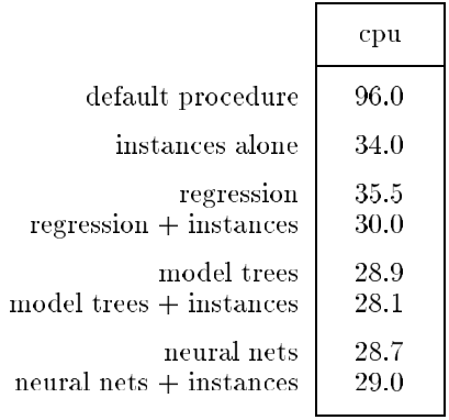
Reference
This is the mean error on unseen data reported in Quinlan (1993) that we use as reference.
Train
This is the score for the opt configuration when
considering the train set.
#plot
renoir:::plot.RenoirSummaryTable(
  x = resl[resl$config == "opt",,drop=F], #select opt config
  measure     = "mae",
  set         = "train",
  interactive = T,
  add.boxplot = F,
  add.scores  = F,
  add.best    = F,
  key         = c("id", "config")
  )
This is the score for the 1se configuration when
considering the train set.
#plot
renoir:::plot.RenoirSummaryTable(
  x = resl[resl$config == "1se",,drop=F], #select 1se config
  measure     = "mae",
  set         = "train",
  interactive = T,
  add.boxplot = F,
  add.scores  = F,
  add.best    = F,
  key         = c("id", "config")
  )
Test
This is the mae score for the opt configuration when
considering the test set.
#plot
renoir:::plot.RenoirSummaryTable(
  x = resl[resl$config == "opt",,drop=F], #select opt config
  measure     = "mae",
  set         = "test",
  interactive = T,
  add.boxplot = F,
  add.scores  = F,
  add.best    = F,
  key         = c("id", "config")
  )
This is the mae score for the 1se configuration when
considering the test set.
#plot
renoir:::plot.RenoirSummaryTable(
  x = resl[resl$config == "1se",,drop=F], #select 1se config
  measure     = "mae",
  set         = "test",
  interactive = T,
  add.boxplot = F,
  add.scores  = F,
  add.best    = F,
  key         = c("id", "config")
  )
Full
This is the mae score for the opt configuration when
considering the full set.
#plot
renoir:::plot.RenoirSummaryTable(
  x = resl[resl$config == "opt",,drop=F], #select opt config
  measure     = "mae",
  set         = "full",
  interactive = T,
  add.boxplot = F,
  add.scores  = F,
  add.best    = F,
  key         = c("id", "config")
  )
This is the mae score for the 1se configuration when
considering the full set.
#plot
renoir:::plot.RenoirSummaryTable(
  x = resl[resl$config == "1se",,drop=F], #select 1se config
  measure     = "mae",
  set         = "full",
  interactive = T,
  add.boxplot = F,
  add.scores  = F,
  add.best    = F,
  key         = c("id", "config")
  )
Mean Squared Error
We consider here the mean squared error.
Train
This is the mse score for the opt configuration when
considering the train set.
#plot
renoir:::plot.RenoirSummaryTable(
  x = resl[resl$config == "opt",,drop=F], #select opt config
  measure     = "mse",
  set         = "train",
  interactive = T,
  add.boxplot = F,
  add.scores  = F,
  add.best    = F,
  key         = c("id", "config")
  )
This is the mse score for the 1se configuration when
considering the train set.
#plot
renoir:::plot.RenoirSummaryTable(
  x = resl[resl$config == "1se",,drop=F], #select 1se config
  measure     = "mse",
  set         = "train",
  interactive = T,
  add.boxplot = F,
  add.scores  = F,
  add.best    = F,
  key         = c("id", "config")
  )
Test
This is the mse score for the opt configuration when
considering the test set.
#plot
renoir:::plot.RenoirSummaryTable(
  x = resl[resl$config == "opt",,drop=F], #select opt config
  measure     = "mse",
  set         = "test",
  interactive = T,
  add.boxplot = F,
  add.scores  = F,
  add.best    = F,
  key         = c("id", "config")
  )
This is the mse score for the 1se configuration when
considering the test set.
#plot
renoir:::plot.RenoirSummaryTable(
  x = resl[resl$config == "1se",,drop=F], #select 1se config
  measure     = "mse",
  set         = "test",
  interactive = T,
  add.boxplot = F,
  add.scores  = F,
  add.best    = F,
  key         = c("id", "config")
  )
Full
This is the mse score for the opt configuration when
considering the full set.
#plot
renoir:::plot.RenoirSummaryTable(
  x = resl[resl$config == "opt",,drop=F], #select opt config
  measure     = "mse",
  set         = "full",
  interactive = T,
  add.boxplot = F,
  add.scores  = F,
  add.best    = F,
  key         = c("id", "config")
  )
This is the mse score for the 1se configuration when
considering the full set.
#plot
renoir:::plot.RenoirSummaryTable(
  x = resl[resl$config == "1se",,drop=F], #select 1se config
  measure     = "mse",
  set         = "full",
  interactive = T,
  add.boxplot = F,
  add.scores  = F,
  add.best    = F,
  key         = c("id", "config")
  )
Auto MPG Data
The city-cycle fuel consumption data was retrieved from the UC Irvine Machine Learning Repository website.
Setup
Learner
We can now create the related ?Learner objects.
#container
learners = list()

#loop
for(learning.method.id in learning.methods.ids){
  #manual setup
  learners[[learning.method.id]] = Learner(
    tuner      = tuner,
    trainer    = Trainer(id = learning.method.id),
    forecaster = Forecaster(id = learning.method.id),
    scorer     = ScorerList(Scorer(id = performance.metric.id.tuning)),
    selector   = Selector(id = learning.method.id),
    recorder   = Recorder(id = learning.method.id, logger = Logger(level = "ALL", verbose = T)),
    marker     = Marker(id = learning.method.id, logger = Logger(level = "ALL", verbose = T)),
    logger     = Logger(level = "ALL")
  )
}
Evaluator
Finally, we need to set up the ?Evaluator.
#Evaluator
evaluator = Evaluator(
  #Sampling strategy: random sampling without replacement
  sampler = Sampler(
    method = "random",
    k = 10L,
    N = as.integer(length(y))
  ),

  #Performance metric
  scorer  = ScorerList(
    Scorer(id = performance.metric.ids.evaluation[1]),
    Scorer(id = performance.metric.ids.evaluation[2])
  )
)
Analysis
Let’s create a directory to store the results.
#define path
outdir = file.path("..", "..", "data-raw", "benchmark", "regression", "gaussian", "auto_mpg", "analysis")

#create if not existing
if(!dir.exists(outdir)){dir.create(path = outdir, showWarnings = F, recursive = T)}
Before running the analysis, we want to set a seed for the random
number generation (RNG). In fact, different R sessions have different
seeds created from current time and process ID by default, and
consequently different simulation results. By fixing a seed we ensure we
will be able to reproduce the results. We can specify a seed by calling
?set.seed.
In the code below, we set a seed before running the analysis for each considered learning method.
#container list
resl = list()

#loop
for(learning.method.id in learning.methods.ids[c(11,12,15,16,17,13,9)]){

  #Each analysis can take hours, so we save data
  #for future faster load

  #path to file
  fp.obj = file.path(outdir, paste0(learning.method.id,".rds"))
  fp.sum = file.path(outdir, paste0("st_",learning.method.id,".rds"))

  #check if exists
  if(file.exists(fp.sum)){
    #load
    cat(paste0("Reading ", learning.method.id, "..."), sep = "")
    resl[[learning.method.id]] = readRDS(file = fp.sum)
    cat("DONE", sep = "\n")
  } else {

    cat(paste("Learning method:", learning.method.id), sep = "\n")

    #Set a seed for RNG
    set.seed(
      #A seed
      seed = 5381L,                   #a randomly chosen integer value
      #The kind of RNG to use
      kind = "Mersenne-Twister",      #we make explicit the current R default value
      #The kind of Normal generation
      normal.kind = "Inversion"       #we make explicit the current R default value
    )

    resl[[learning.method.id]] = renoir(
      # filter,

      #Training set size
      npoints = 5,
      # ngrid,
      nmin = round(nrow(x)/2),

      #Loop
      looper = Looper(),

      #Store
      filename = "renoir",
      outdir   = NULL,
      restore  = TRUE,

      #Learn
      learner   = learners[[learning.method.id]],

      #Evaluate
      evaluator = evaluator,

      #Log
      logger    = Logger(level = "ALL", verbose = T),

      #Data for training
      hyperparameters = get_hp(id = learning.method.id),
      x         = x,
      y         = y,
      weights   = NULL,
      offset    = NULL,
      resp.type = resp.type,

      #space
      rm.call = FALSE,
      rm.fit  = FALSE,

      #Group results
      grouping = TRUE,

      #No screening
      screening = NULL,

      #Remove call from trainer to reduce space
      keep.call = F
    )

    #save
    saveRDS(object = resl[[learning.method.id]], file = fp.obj)

    #create summary table
    resl[[learning.method.id]] = renoir:::summary_table.RenoirList(resl[[learning.method.id]], key = c("id", "config"))

    #save summary table
    saveRDS(object = resl[[learning.method.id]], file = fp.sum)

    #leave space
    cat("\n\n", sep= "\n")
  }
}

#create summary table
resl = do.call(what = rbind, args = c(resl, make.row.names = F, stringsAsFactors = F))
Performance
Let’s now plot the performance metrics for the opt and
1se configurations, considering the train, test, and full
set of data.
Mean Absolute Error
We consider the mean absolute error.
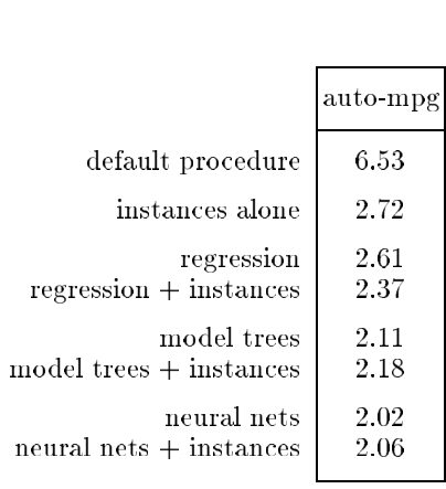
Reference
This is the mean error on unseen data reported in Quinlan (1993) that we use as reference.
Train
This is the score for the opt configuration when
considering the train set.
#plot
renoir:::plot.RenoirSummaryTable(
  x = resl[resl$config == "opt",,drop=F], #select opt config
  measure     = "mae",
  set         = "train",
  interactive = T,
  add.boxplot = F,
  add.scores  = F,
  add.best    = F,
  key         = c("id", "config")
  )
This is the score for the 1se configuration when
considering the train set.
#plot
renoir:::plot.RenoirSummaryTable(
  x = resl[resl$config == "1se",,drop=F], #select 1se config
  measure     = "mae",
  set         = "train",
  interactive = T,
  add.boxplot = F,
  add.scores  = F,
  add.best    = F,
  key         = c("id", "config")
  )
Test
This is the mae score for the opt configuration when
considering the test set.
#plot
renoir:::plot.RenoirSummaryTable(
  x = resl[resl$config == "opt",,drop=F], #select opt config
  measure     = "mae",
  set         = "test",
  interactive = T,
  add.boxplot = F,
  add.scores  = F,
  add.best    = F,
  key         = c("id", "config")
  )
This is the mae score for the 1se configuration when
considering the test set.
#plot
renoir:::plot.RenoirSummaryTable(
  x = resl[resl$config == "1se",,drop=F], #select 1se config
  measure     = "mae",
  set         = "test",
  interactive = T,
  add.boxplot = F,
  add.scores  = F,
  add.best    = F,
  key         = c("id", "config")
  )
Full
This is the mae score for the opt configuration when
considering the full set.
#plot
renoir:::plot.RenoirSummaryTable(
  x = resl[resl$config == "opt",,drop=F], #select opt config
  measure     = "mae",
  set         = "full",
  interactive = T,
  add.boxplot = F,
  add.scores  = F,
  add.best    = F,
  key         = c("id", "config")
  )
This is the mae score for the 1se configuration when
considering the full set.
#plot
renoir:::plot.RenoirSummaryTable(
  x = resl[resl$config == "1se",,drop=F], #select 1se config
  measure     = "mae",
  set         = "full",
  interactive = T,
  add.boxplot = F,
  add.scores  = F,
  add.best    = F,
  key         = c("id", "config")
  )
Mean Squared Error
We consider here the mean squared error.
Train
This is the mse score for the opt configuration when
considering the train set.
#plot
renoir:::plot.RenoirSummaryTable(
  x = resl[resl$config == "opt",,drop=F], #select opt config
  measure     = "mse",
  set         = "train",
  interactive = T,
  add.boxplot = F,
  add.scores  = F,
  add.best    = F,
  key         = c("id", "config")
  )
This is the mse score for the 1se configuration when
considering the train set.
#plot
renoir:::plot.RenoirSummaryTable(
  x = resl[resl$config == "1se",,drop=F], #select 1se config
  measure     = "mse",
  set         = "train",
  interactive = T,
  add.boxplot = F,
  add.scores  = F,
  add.best    = F,
  key         = c("id", "config")
  )
Test
This is the mse score for the opt configuration when
considering the test set.
#plot
renoir:::plot.RenoirSummaryTable(
  x = resl[resl$config == "opt",,drop=F], #select opt config
  measure     = "mse",
  set         = "test",
  interactive = T,
  add.boxplot = F,
  add.scores  = F,
  add.best    = F,
  key         = c("id", "config")
  )
This is the mse score for the 1se configuration when
considering the test set.
#plot
renoir:::plot.RenoirSummaryTable(
  x = resl[resl$config == "1se",,drop=F], #select 1se config
  measure     = "mse",
  set         = "test",
  interactive = T,
  add.boxplot = F,
  add.scores  = F,
  add.best    = F,
  key         = c("id", "config")
  )
Full
This is the mse score for the opt configuration when
considering the full set.
#plot
renoir:::plot.RenoirSummaryTable(
  x = resl[resl$config == "opt",,drop=F], #select opt config
  measure     = "mse",
  set         = "full",
  interactive = T,
  add.boxplot = F,
  add.scores  = F,
  add.best    = F,
  key         = c("id", "config")
  )
This is the mse score for the 1se configuration when
considering the full set.
#plot
renoir:::plot.RenoirSummaryTable(
  x = resl[resl$config == "1se",,drop=F], #select 1se config
  measure     = "mse",
  set         = "full",
  interactive = T,
  add.boxplot = F,
  add.scores  = F,
  add.best    = F,
  key         = c("id", "config")
  )