An introduction to `sigscores`

Introduction

sigscores is an helpful package providing an easy way to compute summary scores for gene signatures.

There is one main function ?computeSigScores, that can be used to compute all the available scores. The scores can be selected via summary score ids (scores argument) or scorers (scorers argument).

Setup

Firstly, we load sigscores and other needed packages:

library(sigscores)

Seed

Now we want to set a seed for the random number generation (RNG). In fact, different R sessions have different seeds created from current time and process ID by default, and consequently different simulation results. By fixing a seed we ensure we will be able to reproduce the results of this vignette. We can specify a seed by calling ?set.seed.

#Set a seed for RNG
set.seed(
  #A seed
  seed = 5381L,                   #a randomly chosen integer value
  #The kind of RNG to use
  kind = "Mersenne-Twister",      #we make explicit the current R default value
  #The kind of Normal generation
  normal.kind = "Inversion"       #we make explicit the current R default value
)

Data

We create now some simulated data to use. For this vignette, we will consider a matrix with 100 genes and 10 samples.

#number of samples
nc = 10
#number of genes
nr = 100
#create matrix
x = matrix(
  data = sample(x = nr*nc),
  nrow = nr,
  ncol = nc,
  dimnames = list(
    paste0("g",seq_len(nr)), 
    paste0("S",seq_len(nc))
  )
)

We can inspect the data by using the ?head function, which returns the first parts of a vector, matrix, table, data frame or function. Let’s print the first 6 rows of our matrix.

#print
head(x = x, n = 6L)
#>     S1  S2  S3  S4  S5  S6  S7  S8  S9 S10
#> g1 993 702 660 854 769 859 940 679 946 218
#> g2 585 620 941 714 994 369 602 506 981 674
#> g3 175 779 984 834 460 292 445 953 491 673
#> g4 778 855 293 140  29 601 980  82 161 115
#> g5 876  32 838  22 803 804 355 663  11 731
#> g6 835 462 894 560 885  88 442 199 541 725

We can now define our gene signature. For example, we can randomly select some genes from the matrix. Let’s select 20 genes.

#number of genes in signature
ng = 20

#select genes
signature = rownames(x)[sample(x = seq_len(nr), size = ng)]

#print
signature
#>  [1] "g12" "g41" "g23" "g59" "g93" "g70" "g51" "g53" "g20" "g72" "g78" "g48"
#> [13] "g67" "g46" "g36" "g7"  "g13" "g15" "g45" "g33"

Data Transformation

We may want to compute some of the scores on transformed data. Users can obviously directly provide the data to work on as x.

However, to facilitate this task, sigscores provides 2 built-in data transformation functions. A list of currently supported data transformers is available through the ?getAvailableDataTransformers function call.

#list transformers
data.transformers = getAvailableDataTransformers()

#print in table
knitr::kable(x = data.transformers)

	id	name
stepFunction	stepFunction	Step Function
quantile	quantile	Quantile Normalization

We can extract the ids by selecting the id column.

#transformer ids
data.transformers.ids = data.transformers$id

#print
print(data.transformers.ids)
#> [1] "stepFunction" "quantile"

The data transformation function can be obtained through the ?getDataTransformer function call. For example, let’s select a step function as data transformer.

#transformer
data.transformer = getDataTransformer(f = 'stepFunction')

#function
data.transformer
#> function (x, y = c(-1, 0, 1), thr = NULL, method = c("median", 
#>     "mean", "mode", "midrange", "trimean", "iqm", "iqr", "mad"), 
#>     by = c("rows", "cols"), na.rm = TRUE) 
#> {
#>     if (isTRUE(is.vector(x))) {
#>         out = stepFunctionTranformationForVector(x = x, y = y, 
#>             thr = thr, method = method, na.rm = na.rm)
#>     }
#>     else if (isTRUE(is.matrix(x))) {
#>         out = stepFunctionTranformationForMatrix(x = x, y = y, 
#>             thr = thr, method = method, by = by, na.rm = na.rm)
#>     }
#>     else {
#>         stop("Error: 'x' class is not supported.\n")
#>     }
#>     return(out)
#> }
#> <bytecode: 0x55acd5e3dff0>
#> <environment: namespace:sigscores>

Looking at the documentation of ?getDataTransformer we can see the function for computing the step function is called ?stepFunctionTranformation, which accepts different arguments. In particular, method indicates the score to be used as threshold in the step function, and by indicates whether to compute the threshold by applying method to rows or columns of x.

We can then use the transformer to create a new data set to be used for the computation of the scores.

#transform data
newx = do.call(
  what = data.transformer, 
  args = list(x = x, method = 'median', by = 'rows')
)

#print
head(x = newx, n = 6L)
#>    S1 S2 S3 S4 S5 S6 S7 S8 S9 S10
#> g1  1 -1 -1  1 -1  1  1 -1  1  -1
#> g2 -1 -1  1  1  1 -1 -1 -1  1   1
#> g3 -1  1  1  1 -1 -1 -1  1 -1   1
#> g4  1  1  1 -1 -1  1  1 -1 -1  -1
#> g5  1 -1  1 -1  1  1 -1 -1 -1   1
#> g6  1 -1  1  1  1 -1 -1 -1 -1   1

Summary Scores

A list of currently supported scores is available through the ?getAvailableScores function call, which returns a table with two columns:

id: the id of the summary score, to be used in the function calls
name: the name of the summary score

#list summary scores
summary.scores = getAvailableScores()

#print in table
knitr::kable(x = summary.scores)

	id	name
sum	sum	Sum
weightedSum	weightedSum	Weighted Sum
mean	mean	Arithmetic Mean
trimmedMean	trimmedMean	Trimmed Mean
weightedMean	weightedMean	Weighted Mean
median	median	Median
mode	mode	Mode
midrange	midrange	Midrange
midhinge	midhinge	Midhinge
trimean	trimean	Trimean
iqr	iqr	Interquartile Range
iqm	iqm	Interquartile Mean
mad	mad	Median Absolute Deviation
aad	aad	Average Absolute Deviation
ssgsea	ssgsea	Single Sample Gene Set Enrichment Analysis
gsva	gsva	Gene Set Variation Analysis
plage	plage	Pathway Level Analysis of Gene Expression
zscore	zscore	Z-Score

As we previously wrote, ?computeSigScores accepts in input summary score ids or scorers.

Score IDs

We can extract the ids by selecting the id column in the previous table.

#summary score ids
summary.scores.ids = summary.scores$id

#print
print(summary.scores.ids)
#>  [1] "sum"          "weightedSum"  "mean"         "trimmedMean"  "weightedMean"
#>  [6] "median"       "mode"         "midrange"     "midhinge"     "trimean"     
#> [11] "iqr"          "iqm"          "mad"          "aad"          "ssgsea"      
#> [16] "gsva"         "plage"        "zscore"

Internally, the score ids are used to create scorers, that will be used for the computation of the scores.

Scorers

Under the hood, sigscores uses scorers, i.e. functions that compute the summary scores. All scorers in sigscores share some common parameters:

x: a (named) numerical vector or matrix
i: a signature
na.rm: a logical value, indicating whether to remove NA values before the computation of the score
...: further parameters to the specific scoring function
transform.fun: it is used to provide a transformation function
transform.args: a list containing the parameters for transform.fun
transform.sub: a logical value indicating whether to transform x after it is subset for the signature i (used to speedup computation, as transformation function should take less time on a reduced data set)

The option of providing a data transformer to a scorer is given to facilitate the application of specific transformation functions to a selected summary measure via an automated process.

We can retrieve a scorer by providing a single score id to the function ?getScorer or multiple ids to ?getScorers. For example, let’s get the scorer for a weighted sum. We know the related score id (i.e. weightedSum) from the table obtained through the ?getAvailableScores function call, so to obtain the scorer we can do:

#get one scorer
scorer = getScorer(score = "weightedSum")

#see function
scorer
#> function (x, i = NULL, w = NULL, na.rm = TRUE, transform.fun = NULL, 
#>     transform.args = list(), transform.sub = F) 
#> {
#>     if (isTRUE(!is.null(transform.fun) && is.function(transform.fun))) {
#>         x = do.call(what = transform.fun, args = c(list(x = x), 
#>             transform.args))
#>     }
#>     if (isTRUE(!is.null(i))) {
#>         x = x[i, , drop = F]
#>         w = w[i]
#>     }
#>     if (isTRUE(!is.null(w))) {
#>         out = w * x
#>     }
#>     else {
#>         out = x
#>     }
#>     out = matrixStats::colSums2(x = out, na.rm = na.rm)
#>     out = unlist(out)
#>     return(out)
#> }
#> <bytecode: 0x55acd7293200>
#> <environment: namespace:sigscores>

Compute the Scores

Finally, we can compute our summary scores.

Using `scores`

The easiest way for doing so is by passing the score ids to the function via the scores argument. Internally, a scoring function is retrieved for each provided score id by calling ?getScorers.

#compute summary scores
scores = sigscores::computeSigScores(
  x      = x,
  i      = signature,
  na.rm  = FALSE,
  scores = summary.scores.ids
)
#> [1] "Calculating ranks..."
#> [1] "Calculating absolute values from ranks..."
#> [1] "Normalizing..."

#print
head(scores)
#>    sampleID   sum weightedSum   mean trimmedMean weightedMean median mode
#> S1       S1 13331       13331 666.55      666.55       666.55  736.5  137
#> S2       S2 12280       12280 614.00      614.00       614.00  623.0  233
#> S3       S3  8242        8242 412.10      412.10       412.10  366.5   13
#> S4       S4 11360       11360 568.00      568.00       568.00  562.0   53
#> S5       S5  8580        8580 429.00      429.00       429.00  323.0   43
#> S6       S6 11137       11137 556.85      556.85       556.85  519.0   77
#>    midrange midhinge  trimean    iqr   iqm      mad    aad      ssgsea
#> S1    557.0  680.375 708.4375 303.25 720.0 180.8772 178.65  0.89773866
#> S2    610.0  594.125 608.5625 389.25 619.3 322.4655 202.80  0.87143168
#> S3    499.0  409.750 388.1250 438.50 373.1 376.5804 242.20 -0.06961626
#> S4    521.5  574.500 568.2500 532.50 567.1 401.7846 271.30  0.71651992
#> S5    478.0  437.500 380.2500 503.50 384.4 297.2613 243.30  0.11853850
#> S6    521.0  547.500 533.2500 387.00 529.9 263.1615 216.75  0.44551534
#>          gsva      plage     zscore
#> S1  0.3540929 -0.3210647  2.1673343
#> S2  0.3861167  0.2938191  1.1924762
#> S3 -0.4555556  0.5088480 -1.9536056
#> S4  0.1970318 -0.1577183  0.4199618
#> S5 -0.1037908  0.1773275 -1.2097106
#> S6  0.1068011 -0.3916968  0.5601269

Using `scorers`

Alternatively, we can define our own list by providing scoring functions. Let’s retrieve two scorers by using the function ?getScorer.

#create scorers list
scorers = list(
  'mean'     = getScorer("mean"),
  'midpoint' = getScorer("median")#we name this score 'midpoint'
)

#compute summary scores
scores = sigscores::computeSigScores(
  x      = x,
  i      = signature,
  na.rm  = T,
  scorers = scorers
)

#print
head(scores)
#>    sampleID   mean midpoint
#> S1       S1 666.55    736.5
#> S2       S2 614.00    623.0
#> S3       S3 412.10    366.5
#> S4       S4 568.00    562.0
#> S5       S5 429.00    323.0
#> S6       S6 556.85    519.0

Changing Default Arguments

To change the default arguments of a specific score function, we can use args: the argument accept a named list, where the name of the element must match the id of the score we want to compute. For example, we may want to compute a trimmed mean considering a specific fraction of elements to be trimmed from each end. Looking at the documentation of ?computeSigScores we can see the scorer computing the trimmed mean is called ?trimmedMeanScorer, which accepts an argument trim. We can then pass the argument from ?computeSigScores via args:

#compute summary scores
scores = sigscores::computeSigScores(
  x      = x,
  i      = signature,
  na.rm  = T,
  scores = summary.scores.ids,
  args   = list(trimmedMean = list(trim = 0.2))
)
#> [1] "Calculating ranks..."
#> [1] "Calculating absolute values from ranks..."
#> [1] "Normalizing..."

#print
head(scores)
#>    sampleID   sum weightedSum   mean trimmedMean weightedMean median mode
#> S1       S1 13331       13331 666.55    712.5833       666.55  736.5  137
#> S2       S2 12280       12280 614.00    615.1667       614.00  623.0  233
#> S3       S3  8242        8242 412.10    376.5833       412.10  366.5   13
#> S4       S4 11360       11360 568.00    568.0833       568.00  562.0   53
#> S5       S5  8580        8580 429.00    395.0000       429.00  323.0   43
#> S6       S6 11137       11137 556.85    543.3333       556.85  519.0   77
#>    midrange midhinge  trimean    iqr   iqm      mad    aad      ssgsea
#> S1    557.0  680.375 708.4375 303.25 720.0 180.8772 178.65  0.89773866
#> S2    610.0  594.125 608.5625 389.25 619.3 322.4655 202.80  0.87143168
#> S3    499.0  409.750 388.1250 438.50 373.1 376.5804 242.20 -0.06961626
#> S4    521.5  574.500 568.2500 532.50 567.1 401.7846 271.30  0.71651992
#> S5    478.0  437.500 380.2500 503.50 384.4 297.2613 243.30  0.11853850
#> S6    521.0  547.500 533.2500 387.00 529.9 263.1615 216.75  0.44551534
#>          gsva      plage     zscore
#> S1  0.3540929 -0.3210647  2.1673343
#> S2  0.3861167  0.2938191  1.1924762
#> S3 -0.4555556  0.5088480 -1.9536056
#> S4  0.1970318 -0.1577183  0.4199618
#> S5 -0.1037908  0.1773275 -1.2097106
#> S6  0.1068011 -0.3916968  0.5601269

`scorers` and `args`

By using scorers and args we can define our list of scorers having specific names and parameters.

#create scorers list
scorers = list(
  'trimmedMean03' = getScorer("trimmedMean"),
  'trimmedMean04' = getScorer("trimmedMean")
)

#compute summary scores
scores2 = sigscores::computeSigScores(
  x      = x,
  i      = signature,
  na.rm  = T,
  scorers = scorers,
  args   = list(
    trimmedMean03 = list(trim = 0.3),
    trimmedMean04 = list(trim = 0.4)
  )
)

#print
head(scores2)
#>    sampleID trimmedMean03 trimmedMean04
#> S1       S1       729.500        736.00
#> S2       S2       625.625        619.00
#> S3       S3       362.625        362.25
#> S4       S4       565.125        559.50
#> S5       S5       372.000        336.50
#> S6       S6       530.750        525.25

Transforming the Data

To facilitate the application of specific transformation functions to selected scores via an automated process, it is possible to provide a data transformer in input to the scorers. The provided transformer is used to transform the data before the computation of the scores.

To pass the needed parameters to the scorer from ?computeSigScores we can again use args.

#Transform data and compute the scores
scoresTD = computeSigScores(
  x = x,
  i = signature,
  scorers = list(
   'score1' = getScorer('weightedSum'),
   'score2' = getScorer('trimmedMean')
  ),
  args = list(
   'score1' = list(
      transform.fun = getDataTransformer('quantile')
    ),
   'score2' = list(
      trim = 0.2,
      transform.fun = getDataTransformer('stepFunction'),
      transform.args = list(
        method = 'median',
        by = 'rows'
      )
    )
  )
)

#print
head(scoresTD)
#>    sampleID  score1     score2
#> S1       S1 12533.2  0.8333333
#> S2       S2 12396.8  0.0000000
#> S3       S3  8713.9 -0.5000000
#> S4       S4 11591.0  0.1666667
#> S5       S5  9712.2 -0.3333333
#> S6       S6 10637.2  0.0000000

Visualisation

sigscores provides some basic functions for plotting. For example, we can plot our computed results via an heat map by using the ?heatmapSigScores function, which requires the output of ?computeSigScores as the data parameter.

#create plot
p = sigscores::heatmapSigScores(
  data   = scores
)

#visualise
p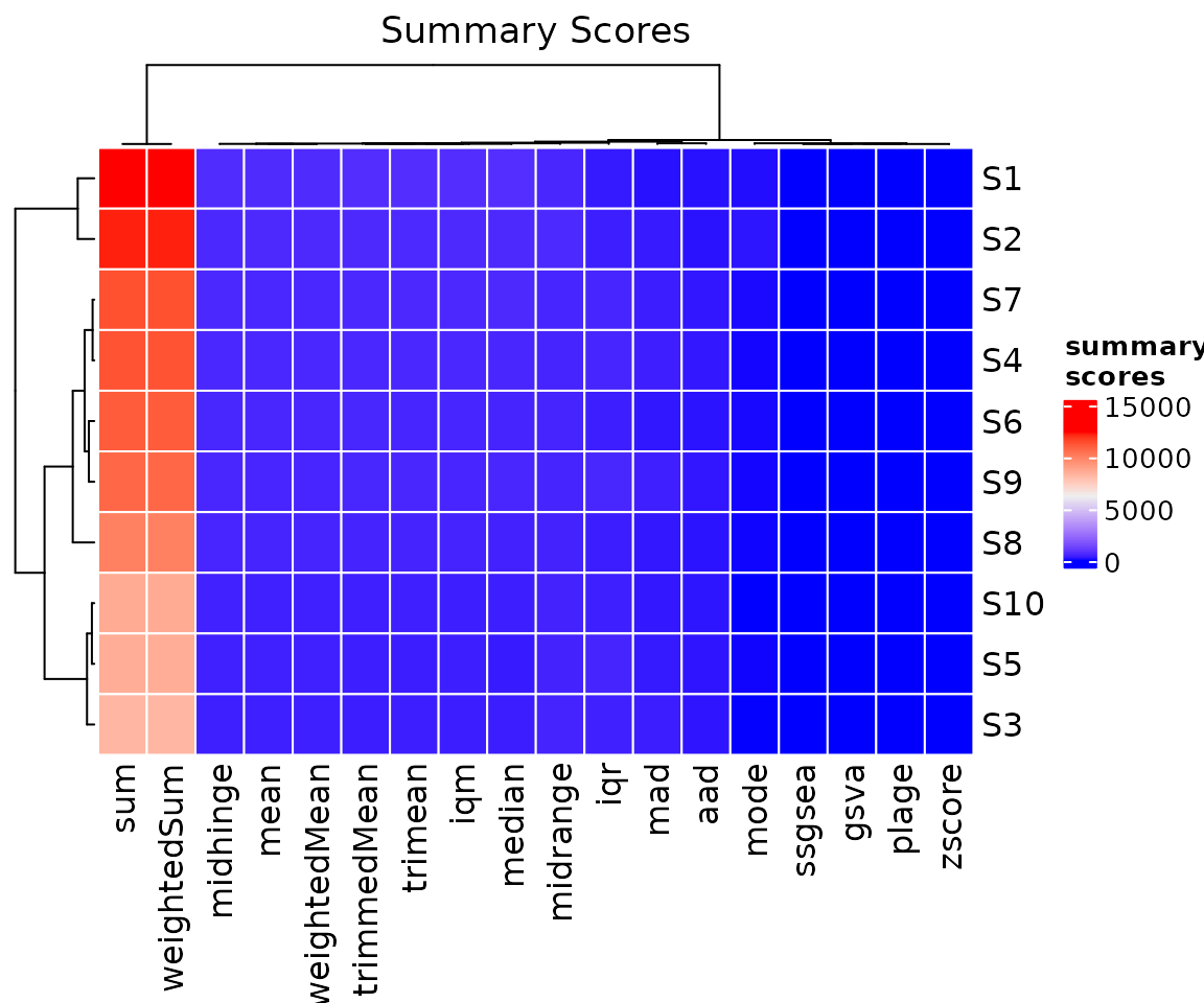

We can visualise the correlation of the summary scores by using another built-in function, i.e. ?heatmapCorSigScores. The correlation matrix can be directly provided via the cor parameter. If cor = NULL, ?heatmapCorSigScores internally computes the correlation by using the default settings of ?computeSigScoresCorrelation.

#create plot
p = sigscores::heatmapCorSigScores(
  data = scores,
  cor  = NULL
)

#visualise
p

It is also possible to represent the summary scores via box plots thanks to another built-in function, i.e. ?boxplotSigScores. We can also subset the scores we want to plot by using the scores parameter.

#create plot
p = sigscores::boxplotSigScores(
  data   = scores,
  scores = c("mean", "mode", "median", "iqm", "midrange", "midhinge", "trimean")
)

#visualise
p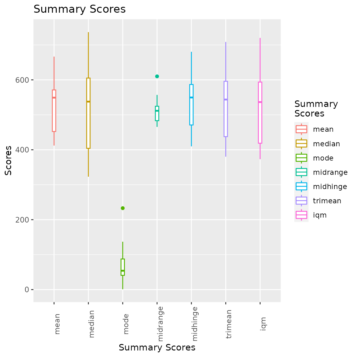
#> Warning: Use of `data[[x]]` is discouraged.
#> ℹ Use `.data[[x]]` instead.
#> Warning: Use of `data[[y]]` is discouraged.
#> ℹ Use `.data[[y]]` instead.
#> Warning: Use of `data[[color]]` is discouraged.
#> ℹ Use `.data[[color]]` instead.

Significance of the Scores

We may want to understand if the computed scores are due to the selected genes in our signature, or if we might have ended up with similar scores also with different lists of genes.

Sampling the Data

To associate significance to each of the computed scores we can use a resampling method. The idea is to calculate the probability of observing a resampling value as extreme as the one calculated on the original data. The main steps involved in this process are:

Draw random samples from the original data
Compute the summary scores on the simulated data
Create a sampling distribution for each score
Calculate the significance for each score

To facilitate this computation, ?computeSigScores can also calculate the summary scores for data sets generated using resampling. Two techniques are provided out-of-the-box in ?computeSigScores: permutation (i.e. sampling without replacement) and bootstrap (i.e. sampling with replacement). The main new arguments we need to set are sampling, which indicates the technique we want to use, and n.repeat, which tells the function how many random samples we want to generate.

Let’s create summary scores for 10 data sets generated using sampling without replacement.

#compute summary scores
scores = sigscores::computeSigScores(
  x        = x,
  i        = signature,
  na.rm    = F,
  scores   = summary.scores.ids,
  sampling = "permutation",
  n.repeat = 10
)
#> [1] "Calculating ranks..."
#> [1] "Calculating absolute values from ranks..."
#> [1] "Normalizing..."
#> [1] "Calculating ranks..."
#> [1] "Calculating absolute values from ranks..."
#> [1] "Normalizing..."
#> [1] "Calculating ranks..."
#> [1] "Calculating absolute values from ranks..."
#> [1] "Normalizing..."
#> [1] "Calculating ranks..."
#> [1] "Calculating absolute values from ranks..."
#> [1] "Normalizing..."
#> [1] "Calculating ranks..."
#> [1] "Calculating absolute values from ranks..."
#> [1] "Normalizing..."
#> [1] "Calculating ranks..."
#> [1] "Calculating absolute values from ranks..."
#> [1] "Normalizing..."
#> [1] "Calculating ranks..."
#> [1] "Calculating absolute values from ranks..."
#> [1] "Normalizing..."
#> [1] "Calculating ranks..."
#> [1] "Calculating absolute values from ranks..."
#> [1] "Normalizing..."
#> [1] "Calculating ranks..."
#> [1] "Calculating absolute values from ranks..."
#> [1] "Normalizing..."
#> [1] "Calculating ranks..."
#> [1] "Calculating absolute values from ranks..."
#> [1] "Normalizing..."

#print
head(scores)
#>   run sampleID   sum weightedSum   mean trimmedMean weightedMean median mode
#> 1   1       S1  7277        7277 363.85      363.85       363.85  261.0    2
#> 2   1       S2  9930        9930 496.50      496.50       496.50  507.5    3
#> 3   1       S3  8750        8750 437.50      437.50       437.50  384.0   81
#> 4   1       S4  9134        9134 456.70      456.70       456.70  399.0   51
#> 5   1       S5  7427        7427 371.35      371.35       371.35  319.0    8
#> 6   1       S6 11418       11418 570.90      570.90       570.90  571.0  149
#>   midrange midhinge  trimean    iqr   iqm      mad    aad      ssgsea
#> 1    449.0  357.750 309.3750 641.50 305.3 352.1175 285.95 -0.49970900
#> 2    489.0  489.250 498.3750 356.50 489.6 283.9179 215.40  0.19929221
#> 3    539.0  372.500 378.2500 408.00 357.4 346.9284 259.30  0.01770463
#> 4    520.5  479.875 439.4375 343.25 432.2 293.5548 214.10  0.11019309
#> 5    454.0  379.750 349.3750 432.00 336.9 302.4504 223.85 -0.21291592
#> 6    557.0  552.125 561.5625 430.25 574.7 349.8936 225.40  0.49461406
#>         gsva        plage     zscore
#> 1 -0.3371350 -0.430876879 -1.3739329
#> 2  0.1311368 -0.002122875  0.3751179
#> 3  0.1157828 -0.385513783 -0.8065714
#> 4  0.1502551 -0.088276998 -0.1428458
#> 5 -0.1771978 -0.209271662 -1.3765625
#> 6  0.4529517  0.453742266  1.6396185

To use bootstrap instead, we just need change the sampling argument.

#compute summary scores
scores = sigscores::computeSigScores(
  x        = x,
  i        = signature,
  na.rm    = F,
  scores   = summary.scores.ids,
  sampling = "bootstrap",
  n.repeat = 10
)
#> [1] "Calculating ranks..."
#> [1] "Calculating absolute values from ranks..."
#> [1] "Normalizing..."
#> [1] "Calculating ranks..."
#> [1] "Calculating absolute values from ranks..."
#> [1] "Normalizing..."
#> [1] "Calculating ranks..."
#> [1] "Calculating absolute values from ranks..."
#> [1] "Normalizing..."
#> [1] "Calculating ranks..."
#> [1] "Calculating absolute values from ranks..."
#> [1] "Normalizing..."
#> [1] "Calculating ranks..."
#> [1] "Calculating absolute values from ranks..."
#> [1] "Normalizing..."
#> [1] "Calculating ranks..."
#> [1] "Calculating absolute values from ranks..."
#> [1] "Normalizing..."
#> [1] "Calculating ranks..."
#> [1] "Calculating absolute values from ranks..."
#> [1] "Normalizing..."
#> [1] "Calculating ranks..."
#> [1] "Calculating absolute values from ranks..."
#> [1] "Normalizing..."
#> [1] "Calculating ranks..."
#> [1] "Calculating absolute values from ranks..."
#> [1] "Normalizing..."
#> [1] "Calculating ranks..."
#> [1] "Calculating absolute values from ranks..."
#> [1] "Normalizing..."

#print
head(x = scores, n = 6L)
#>   run sampleID   sum weightedSum   mean trimmedMean weightedMean median mode
#> 1   1       S1 10628       10628 531.40      531.40       531.40  692.0  692
#> 2   1       S2  9163        9163 458.15      458.15       458.15  361.5   32
#> 3   1       S3 10665       10665 533.25      533.25       533.25  584.5  563
#> 4   1       S4  7325        7325 366.25      366.25       366.25  409.5   22
#> 5   1       S5  8657        8657 432.85      432.85       432.85  400.5    6
#> 6   1       S6 11009       11009 550.45      550.45       550.45  566.0  566
#>   midrange midhinge  trimean    iqr   iqm      mad    aad     ssgsea
#> 1    440.5  510.500 601.2500 524.50 601.4 262.4202 246.90  0.2382717
#> 2    503.5  478.125 419.8125 536.25 416.0 325.4307 258.95  0.2153395
#> 3    539.0  510.375 547.4375 590.75 545.3 404.0085 259.25  0.3853388
#> 4    420.0  339.500 374.5000 321.00 383.7 186.0663 181.45 -0.2816480
#> 5    472.0  437.625 419.0625 637.25 439.1 524.0991 305.45  0.1844530
#> 6    560.5  564.500 565.2500 479.00 559.7 352.8588 229.95  0.4535682
#>          gsva       plage     zscore
#> 1  0.10920578 -0.15801753  0.8728117
#> 2  0.07273132  0.42059271 -0.5968935
#> 3  0.10535714 -0.26930515  0.4721479
#> 4 -0.19861111  0.05836157 -1.3292259
#> 5 -0.16397300 -0.53494029 -0.4985339
#> 6  0.17213115  0.00608184  0.7195745

Random Signatures

Instead of creating new data sets via resampling, we can also generate random signatures, i.e. randomly generated vectors of the same size as i.

To facilitate this computation, ?computeSigScoresallows two options: rndsig (where all elements - row indices - of x can be randomly selected) and rndsigsub (where only the elements - row indices - of x that are not in i can be randomly selected). We can still use the sampling parameter to indicate the technique we want to use, and n.repeat, to tell the function how many random signatures we want to generate.

Let’s create summary scores for 10 random signatures. For doing so, we just need to write sampling = 'rndsig'.

#compute summary scores
scores = sigscores::computeSigScores(
  x        = x,
  i        = signature,
  na.rm    = T,
  scores   = summary.scores.ids,
  sampling = "rndsig",
  n.repeat = 10
)
#> [1] "Calculating ranks..."
#> [1] "Calculating absolute values from ranks..."
#> [1] "Normalizing..."
#> [1] "Calculating ranks..."
#> [1] "Calculating absolute values from ranks..."
#> [1] "Normalizing..."
#> [1] "Calculating ranks..."
#> [1] "Calculating absolute values from ranks..."
#> [1] "Normalizing..."
#> [1] "Calculating ranks..."
#> [1] "Calculating absolute values from ranks..."
#> [1] "Normalizing..."
#> [1] "Calculating ranks..."
#> [1] "Calculating absolute values from ranks..."
#> [1] "Normalizing..."
#> [1] "Calculating ranks..."
#> [1] "Calculating absolute values from ranks..."
#> [1] "Normalizing..."
#> [1] "Calculating ranks..."
#> [1] "Calculating absolute values from ranks..."
#> [1] "Normalizing..."
#> [1] "Calculating ranks..."
#> [1] "Calculating absolute values from ranks..."
#> [1] "Normalizing..."
#> [1] "Calculating ranks..."
#> [1] "Calculating absolute values from ranks..."
#> [1] "Normalizing..."
#> [1] "Calculating ranks..."
#> [1] "Calculating absolute values from ranks..."
#> [1] "Normalizing..."

#print
head(x = scores, n = 6L)
#>   run sampleID   sum weightedSum   mean trimmedMean weightedMean median mode
#> 1   1       S1 10642       10642 532.10      532.10       532.10  625.5    2
#> 2   1       S2  9849        9849 492.45      492.45       492.45  549.5    3
#> 3   1       S3 10235       10235 511.75      511.75       511.75  458.5   25
#> 4   1       S4  7217        7217 360.85      360.85       360.85  365.0   12
#> 5   1       S5  7658        7658 382.90      382.90       382.90  320.5    6
#> 6   1       S6 10667       10667 533.35      533.35       533.35  508.5  159
#>   midrange midhinge  trimean    iqr   iqm      mad    aad     ssgsea
#> 1    497.5  452.000 538.7500 556.50 578.0 282.4353 250.40  0.2919138
#> 2    435.0  489.250 519.3750 432.50 544.7 243.1464 217.45  0.3374312
#> 3    511.0  504.625 481.5625 343.75 515.0 347.6697 249.55  0.4744933
#> 4    433.0  318.250 341.6250 504.50 329.8 347.6697 230.15 -0.4304196
#> 5    459.5  356.000 338.2500 511.50 349.9 395.8542 265.40 -0.0516426
#> 6    579.5  509.875 509.1875 330.75 510.7 268.3506 197.45  0.2885531
#>          gsva       plage      zscore
#> 1 -0.04816398 -0.43202354  0.67191640
#> 2 -0.02836022  0.29436181  0.06091783
#> 3  0.13897059  0.19256993  0.05269303
#> 4 -0.43261278  0.01629289 -1.81167058
#> 5 -0.21453831 -0.27036762 -1.47974905
#> 6  0.13154206  0.02685464  0.59379833

A final available option is to generate random signatures by using all possible elements of x after removing the value from i. For this scenario, we just need to use sampling = 'rndsigsub'.

#compute summary scores
scores = sigscores::computeSigScores(
  x        = x,
  i        = signature,
  na.rm    = T,
  scores   = summary.scores.ids,
  sampling = "rndsigsub",
  n.repeat = 10
)
#> [1] "Calculating ranks..."
#> [1] "Calculating absolute values from ranks..."
#> [1] "Normalizing..."
#> [1] "Calculating ranks..."
#> [1] "Calculating absolute values from ranks..."
#> [1] "Normalizing..."
#> [1] "Calculating ranks..."
#> [1] "Calculating absolute values from ranks..."
#> [1] "Normalizing..."
#> [1] "Calculating ranks..."
#> [1] "Calculating absolute values from ranks..."
#> [1] "Normalizing..."
#> [1] "Calculating ranks..."
#> [1] "Calculating absolute values from ranks..."
#> [1] "Normalizing..."
#> [1] "Calculating ranks..."
#> [1] "Calculating absolute values from ranks..."
#> [1] "Normalizing..."
#> [1] "Calculating ranks..."
#> [1] "Calculating absolute values from ranks..."
#> [1] "Normalizing..."
#> [1] "Calculating ranks..."
#> [1] "Calculating absolute values from ranks..."
#> [1] "Normalizing..."
#> [1] "Calculating ranks..."
#> [1] "Calculating absolute values from ranks..."
#> [1] "Normalizing..."
#> [1] "Calculating ranks..."
#> [1] "Calculating absolute values from ranks..."
#> [1] "Normalizing..."

#print
head(x = scores, n = 6L)
#>   run sampleID   sum weightedSum   mean trimmedMean weightedMean median mode
#> 1   1       S1 10228       10228 511.40      511.40       511.40  540.5   23
#> 2   1       S2  8830        8830 441.50      441.50       441.50  410.0  139
#> 3   1       S3  7995        7995 399.75      399.75       399.75  312.0   81
#> 4   1       S4 10317       10317 515.85      515.85       515.85  441.5   12
#> 5   1       S5  8570        8570 428.50      428.50       428.50  391.5   46
#> 6   1       S6 12061       12061 603.05      603.05       603.05  648.5  159
#>   midrange midhinge  trimean    iqr   iqm      mad    aad      ssgsea
#> 1    470.5  537.750 539.1250 321.00 516.0 243.1464 209.10  0.03927932
#> 2    505.5  425.000 417.5000 330.00 426.8 269.8332 189.60 -0.24184922
#> 3    493.0  428.250 370.1250 445.00 340.8 237.9573 217.55 -0.28906294
#> 4    501.0  524.125 482.8125 361.25 495.0 295.7787 233.35  0.45904479
#> 5    502.5  420.000 405.7500 532.50 406.6 413.6454 283.70  0.15920415
#> 6    574.0  607.500 628.0000 289.50 614.3 254.2659 193.15  0.71093706
#>          gsva       plage     zscore
#> 1 -0.06704545  0.16191884  0.2105943
#> 2 -0.32649083  0.04897823 -0.8893993
#> 3 -0.27180353 -0.17507515 -1.6517839
#> 4  0.21018271  0.24197781  0.4720690
#> 5 -0.06120304  0.48313859 -0.5202871
#> 6  0.37782977 -0.41419008  1.6535733

Logging

sigscores provides a basic event logging system. It can be easily set-up by providing a ?Logger to ?computeSigScores. A ?Logger can be created by calling the ?createLogger function.

#compute summary scores
scores = sigscores::computeSigScores(
  x        = x,
  i        = signature,
  na.rm    = T,
  scores   = summary.scores.ids,
  logger   = createLogger(verbose = TRUE, level = "DEBUG")
)
#> [INFO]  2023-02-02 12:27:23 SIGSCORES
#> [DEBUG] 2023-02-02 12:27:23 Starting the computation.
#> ------------------------------------------
#> [DEBUG] 2023-02-02 12:27:23 Iteration 1
#> [DEBUG] 2023-02-02 12:27:23 Iteration 2
#> [DEBUG] 2023-02-02 12:27:23 Iteration 3
#> [DEBUG] 2023-02-02 12:27:23 Iteration 4
#> [DEBUG] 2023-02-02 12:27:23 Iteration 5
#> [DEBUG] 2023-02-02 12:27:23 Iteration 6
#> [DEBUG] 2023-02-02 12:27:23 Iteration 7
#> [DEBUG] 2023-02-02 12:27:23 Iteration 8
#> [DEBUG] 2023-02-02 12:27:23 Iteration 9
#> [DEBUG] 2023-02-02 12:27:23 Iteration 10
#> [DEBUG] 2023-02-02 12:27:23 Iteration 11
#> [DEBUG] 2023-02-02 12:27:23 Iteration 12
#> [DEBUG] 2023-02-02 12:27:23 Iteration 13
#> [DEBUG] 2023-02-02 12:27:23 Iteration 14
#> [DEBUG] 2023-02-02 12:27:23 Iteration 15
#> [1] "Calculating ranks..."
#> [1] "Calculating absolute values from ranks..."
#> [1] "Normalizing..."
#> [DEBUG] 2023-02-02 12:27:23 Iteration 16
#> [DEBUG] 2023-02-02 12:27:23 Iteration 17
#> [DEBUG] 2023-02-02 12:27:23 Iteration 18
#> ------------------------------------------
#> [DEBUG] 2023-02-02 12:27:23 Computation finished.
#> [DEBUG] 2023-02-02 12:27:23 Creating output object...DONE

Save to File

The result of the computation and a log file can be automatically saved to disk.

#define your output directory
outdir = "mydir/test"
#choose a name for the result file
#(without file extension)
resfile = "sigscores"
#choose a name for the log file
#(with file extension)
logfile = "log.txt"
#compute summary scores
scores = sigscores::computeSigScores(
  x        = x,
  i        = signature,
  na.rm    = T,
  scores   = summary.scores.ids,
  logger   = createLogger(
    verbose = TRUE, 
    level   = "DEBUG",
    path    = file.path(outdir, logfile)
  ),
  outdir   = outdir,
  filename = resfile
)

Parallel Execution

sigscores provides a simple approach to speed up computation on a multi-core computer via the usage of parallel, doParallel, and foreach R packages.

To enable parallel execution we just need to set the argument cores in the ?computeSigScores function with an integer greater than 1. For example, let’s try to use 2 cores.

#compute summary scores with parallel execution
scores = sigscores::computeSigScores(
  x        = x,
  i        = signature,
  na.rm    = T,
  scores   = summary.scores.ids,
  sampling = "permutation",
  n.repeat = 2,
  cores    = 2
)

As a note, the function internally perform some checks before setting a parallel environment, so if the provided number of cores is too high it will set cores as the maximum number of available (logical) processors on the machine minus 1.

Serial vs Parallel

We could see the advantage of using a parallel execution by comparing the computation time between a serial and parallel setting when having an higher number of repeats. To time the execution of the function calls we can use the ?system.time R function.

Let’s consider 500 permutations of the original data and compute the scores in a serial fashion first.

#compute summary scores
time_serial = system.time(
  expr = {
    scoresS = sigscores::computeSigScores(
      x        = x,
      i        = signature,
      na.rm    = T,
      scores   = summary.scores.ids,
      sampling = "permutation",
      n.repeat = 500
    )
  }
)

Now we can run the parallel execution with the same number of repeats and selecting 5 cores.

#compute summary scores
time_parallel = system.time(
  expr = {
    scoresP = sigscores::computeSigScores(
      x        = x,
      i        = signature,
      na.rm    = T,
      scores   = summary.scores.ids,
      sampling = "permutation",
      n.repeat = 500,
      cores    = 5
    )
  }
)

Finally, we can compare the execution time. On a laptop having the following hardware:

Intel(R) Core(TM) i7-8650 CPU @ 1.90GHz, 2112MHz, 4 Core(s), 8 Logical Processor(s)
1TB SSD Hard Drive
16GB RAM

the execution times for the serial and parallel computations were:

#create a matrix
m = rbind(
  serial   = time_serial,
  parallel = time_parallel
)

#print
print(m)
#>          user.self sys.self elapsed user.child sys.child
#> serial      170.17     0.06  170.50         NA        NA
#> parallel      1.20     2.08   84.03         NA        NA

The parallel execution was around 2.03 times faster than the serial execution.